Power Query lets you perform a series of steps to transform your Excel data. One of the steps it allows you to take is to fill data down easily.
You might be wondering when you might need to fill data down in your table.
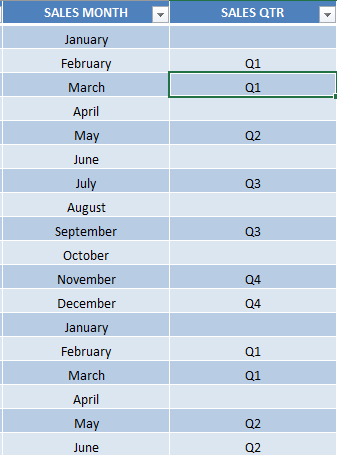
Let’s suppose you have this set of data:
A lot of values are missing in the Sales Quarter column! It would be a lot of effort to input them one by one.
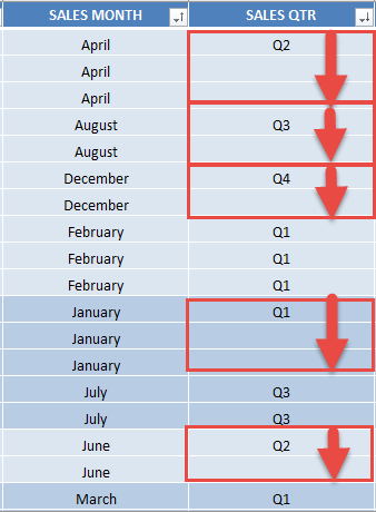
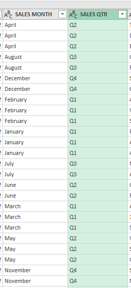
Let us sort the Sales Month, then the Sales Quarter column to get a better understanding:
You can see that we have at least one sales quarter populated for each month.
The technique here is that the Fill Down will copy the value directly above the empty cell and then fill it down the succeeding empty cell.
You can see from the arrows what will happen once we use Fill Down in Power Query.
Now that you know what our game plan is, let us get started!
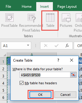
STEP 1: Select your data and turn it into an Excel Table by pressing the shortcut Ctrl + T or by going to Insert > Table
STEP 2: Go to Data > Get & Transform > From Table (Excel 2016) or Power Query > Excel Data > From Table (Excel 2013 & 2010)
Excel 2016:
Excel 2013 & 2010:
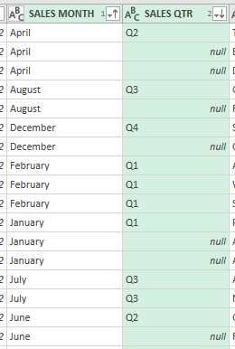
STEP 3: This will open up the Power Query Editor.
A) Sort the Sales Month by Ascending order.
B) Then sort the Sales Quarter by Descending order.
Our data is now ready for the Fill down step.
STEP 4: Make sure the Sales Quarter column is selected. Go to Transform > Fill > Down
The missing values are now populated!
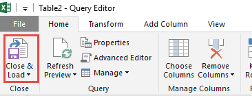
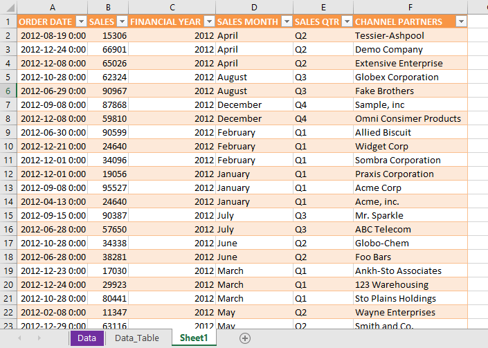
STEP 5: Click Close & Load from the Home tab and this will open up a brand new worksheet in your Excel workbook with the updated values.
You now have your new table with the updated values.
Bryan
Bryan is a best-selling book author of the 101 Excel Series paperback books.
