In Excel you can have a data set that comes from an external source which isn’t always formatted to your liking.
One of the most common things you may encounter are blank cells in your Excel data which can hinder your analysis, especially if you are using a Pivot Table to analyze the data.
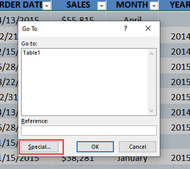
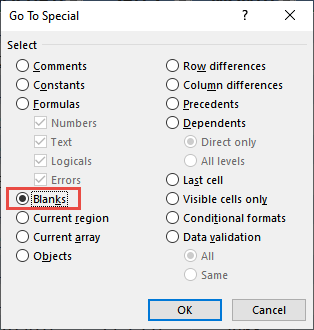
To find these annoying blank cells in Excel you will need to highlight all your data set (CTRL+*) and bring up the Go To shortcut: CTRL+G > Special > Blanks.
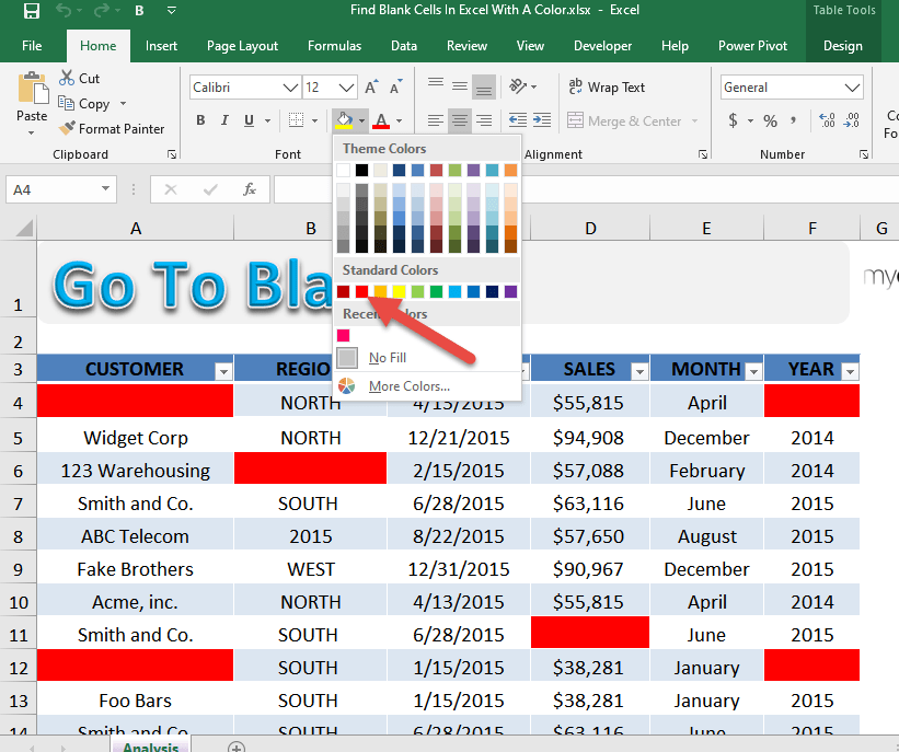
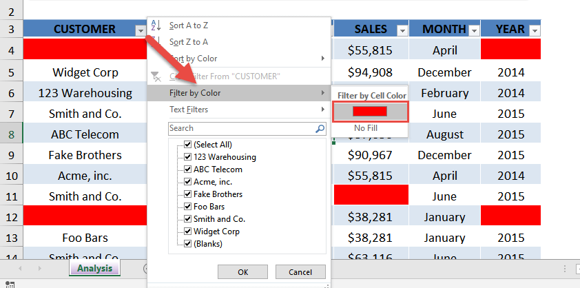
Then you can fill in the blank cells with a color red and filter by that same color to drill down to these blank cells and take some formatting action.
I show you how easy this can be done below.
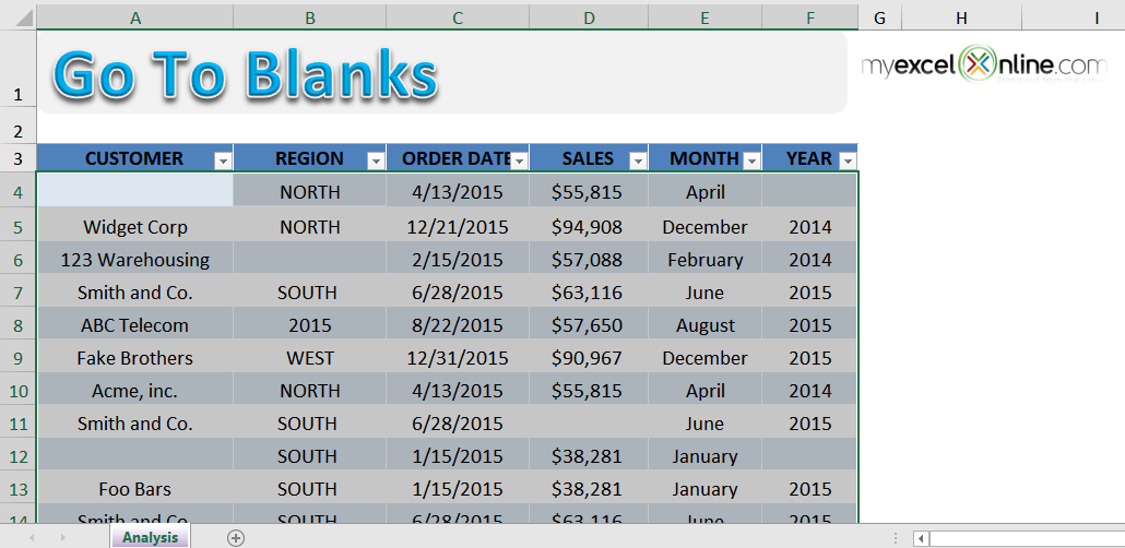
STEP 1: Make sure your entire table is selected. We will select all the blank cells.
STEP 2: Press Ctrl + G to open the Go To Window. Click Special.
Select Blanks. Click OK.
STEP 3: The blank cells are now selected. Go to Home > Font > Fill > Color Red
STEP 4: Let us try it out! Try filtering the Customer column by selecting Filter by Color > Color Red
Our filtering has worked to show the blank cells!
How to Find Blank Cells In Excel With A Color
HELPFUL RESOURCE:
John Michaloudis is a former accountant and finance analyst at General Electric, a Microsoft MVP since 2020, an Amazon #1 bestselling author of 4 Microsoft Excel books and teacher of Microsoft Excel & Office over at his flagship Academy Online Course.

