Finding unique values in Microsoft Excel is essential for data integrity and efficiency, especially when dealing with extensive datasets like customer databases or inventory lists. By leveraging Excel’s functionality to find unique values, users can significantly enhance their data analysis and decision-making processes. Excel provides various methods suitable for different data sets, ensuring flexibility and precision in data management.
5 Key Takeaways
- Excel’s UNIQUE function, combined with SORT, streamlines the creation of ordered, non-duplicate lists, vital for clear reporting and organized drop-down lists.
- Utilize the Advanced Filter feature to efficiently filter unique records in extensive spreadsheets, transforming bulky data into concise, analyzable lists.
- Combine UNIQUE with FILTER to exclude blank cells from your unique values list, ensuring cleaner and more accurate data presentation.
- Use the UNIQUE function to extract unique values across multiple columns, simplifying data analysis by consolidating diverse data points into a cohesive list.
Unlocking Excel’s Potential with Unique Values
The Importance of Identifying Unique Data
Identifying unique data in Excel is critical for maintaining data integrity, and eliminating unnecessary data redundancies can be incredibly beneficial. Whether sorting through extensive customer databases, analyzing results from a comprehensive survey, or managing complex inventory lists, pinpointing those one-of-a-kind entries ensures your analysis is precise and your outcomes are reliable.
Embracing unique values as part of your daily workflow can significantly optimize how you interact with and understand data, leading to more informed and accurate decision-making processes.
Diverse Methods for Different Data Sets
Depending on the nature and complexity of the data set, Excel offers a plethora of methods to help manage and find unique values. Pivot tables might be a go-to strategy for larger, more complex data sets, providing a high-level view of the distinct aspects of your data.
For simpler tasks, functions like UNIQUE() or conditional formatting could be more fit-for-purpose, offering a quick and effective way to filter through data. Each method has its own strengths, allowing you to tailor your approach to meet the specific challenges and nuances of your data set.
Harnessing Key Functions for Uniqueness
The Power of the UNIQUE Function
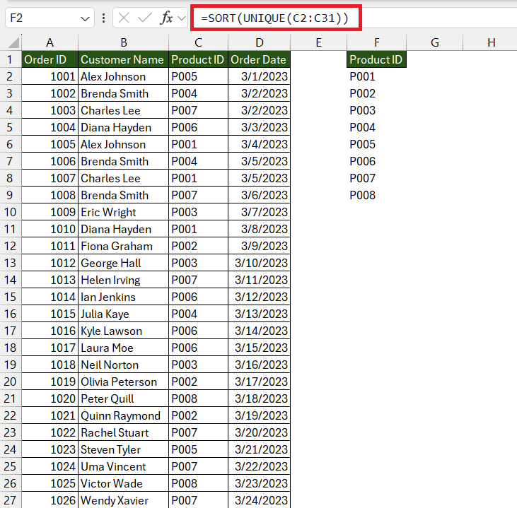
Creating a clean, sorted list of non-duplicate items eliminates confusion and streamlines the data analysis process. To achieve this in Excel, you can blend the UNIQUE function with the SORT function. These two complement each other seamlessly to produce a list that’s both free of repetitions and ordered.
Implement this in the following way:
=SORT(UNIQUE(range))
What happens here is that the UNIQUE function firstly isolates the one-off items from your designated range. Then, the SORT function steps in to put these unique values in order, be it numerical or alphabetical. This duo works wonders, especially when prepping data for clear, comprehensible reporting or when constructing drop-down lists where order and uniqueness are paramount.
Filtering Unique Records in Large Data Sets
When you’re faced with a sprawling spreadsheet full of data, filtering for unique records can feel like finding a needle in a haystack. However, Excel is equipped with tools that streamline this process. The ‘Advanced Filter’ is particularly valuable for sifting through large datasets efficiently. Here’s how to use it for unique records:
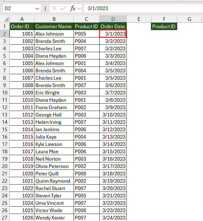
STEP 1: Click a cell within your data set.
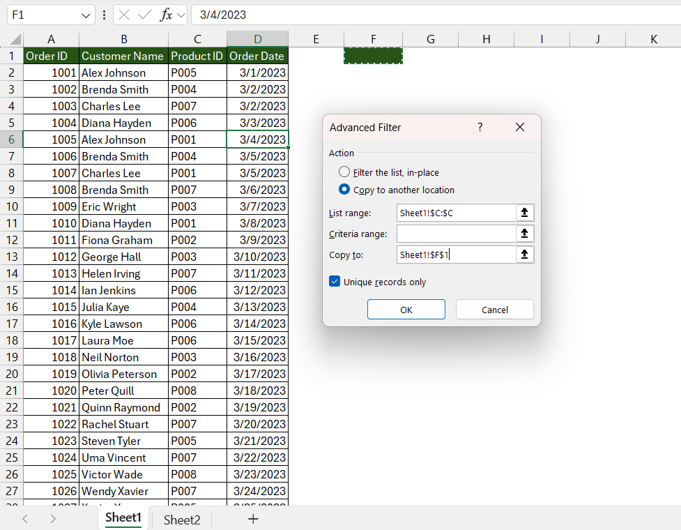
STEP 2: On the Data tab, select ‘Advanced’ in the Sort & Filter group.
STEP 3: Follow the actions below –
- Select the Product ID column as ‘List Range’.
- Opt for ‘Copy to another location’.
- Select cell F1 as ‘Copy to’.
- Check the box for ‘Unique records only’.
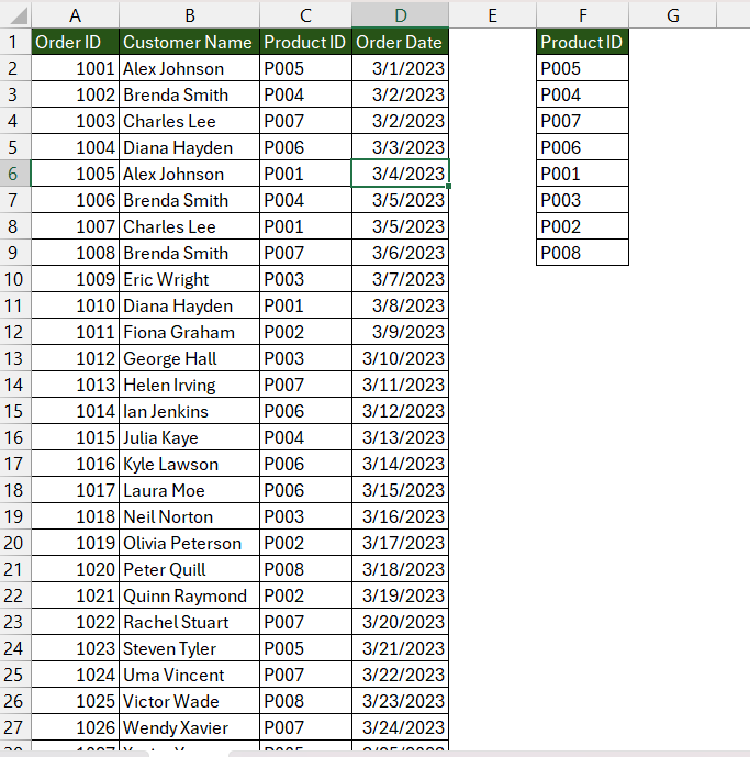
STEP 4: Click OK, and voila, your worksheet now reflects only unique records.
By employing the Advanced Filter, you can instantly transform an overwhelming array of data into a distilled list of unique entries, crucial for in-depth analysis or report generation. Remember, this is particularly useful when working with datasets that are too large for manual sifting.
A Deeper Dive into Formulas and Functions
Unique values in Excel ignoring blanks
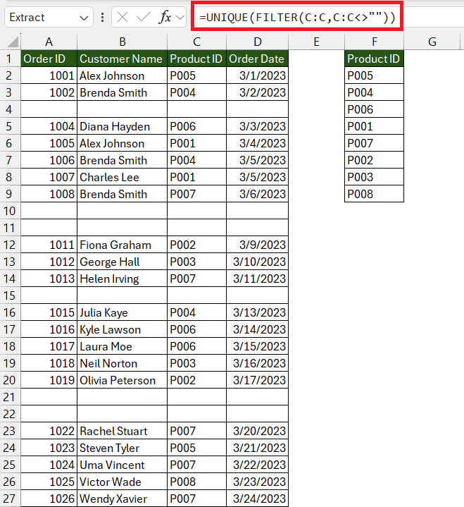
To extract unique values while ignoring blanks in Excel, you’ll want to effectively combine the UNIQUE and FILTER functions. As noted previously, the UNIQUE function instinctively includes all distinct entries, but it doesn’t discriminate against blank cells. However, introducing the FILTER function allows you to sidestep this issue seamlessly.
You’ll craft a formula that filters out any blanks before passing the result to the UNIQUE function:
The FILTER function ensures that any cell that isn’t empty ("") is included, and then UNIQUE comes into play, ensuring that the result consists solely of non-repetitive values, minus the blank cells. This refined list enables cleaner data analysis and presentation, preventing any misleading gaps in your results.
Extracting Unique Values from Multiple Columns
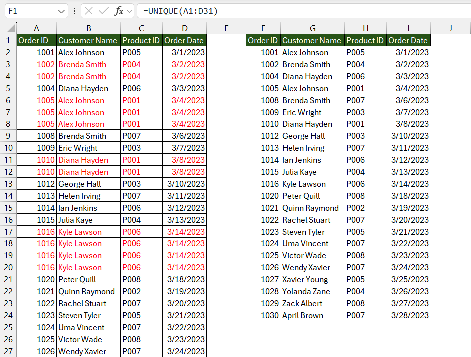
Extracting unique values across multiple columns is a common need in data analysis, as it helps condense a data set into a more manageable and discernible form. Excel simplifies this task with the UNIQUE function, extending its capability beyond single columns to embrace entire ranges, whether vertical or horizontal.
Consider a scenario where you need to pull unique values from a dataset spanning several columns:
This formula jets through cells A1 to D31, sifting out distinct values from the combined columns. The result is a streamlined list representing the intersection of these columns, purged of repeated items. It’s a direct and efficient strategy to garner a comprehensive understanding of multiple data columns without toggling between them.
Tips, Tricks, and Troubleshooting
Overcoming the Dreaded #NAME? Error
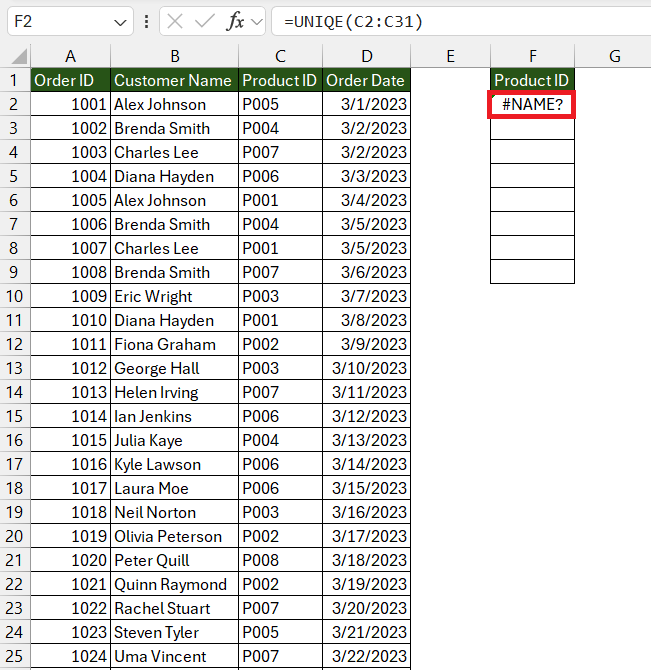
Encountering the #NAME? error can feel like hitting a roadblock, but it’s often a quick fix. This error usually pops up when Excel doesn’t recognize text in the formula—often because of a typo or because the function isn’t supported in your Excel version.
To resolve it, check the spelling of your function first. For instance, if UNIQUE is misspelled, Excel can’t proceed with the operation. Simply correcting the function name should clear things up.
If your version of Excel doesn’t feature UNIQUE, alternative methods like using the Advanced Filter or creating your own unique value generator with combinations of IF, COUNTIF, and array formulas might be necessary.
The #NAME? error is your clue to scrutinize the syntax and compatibility of your functions, ensuring they’re in line with what Excel anticipates.
Dynamic Arrays and #SPILL Errors Explained
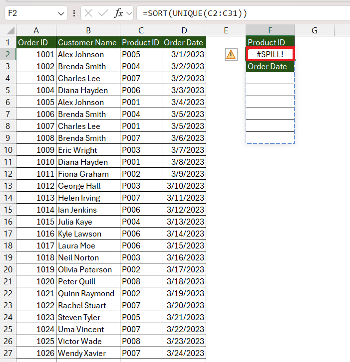
A #SPILL! error occurs if one or more cells in the intended spill range are occupied.
To pinpoint the issue, Excel offers a way to click the error and select ‘Select Obstructing Cells’ to identify and clear them. Always ensure that the spill range is clear of any data or formatting to allow arrays to display their results fully.
FAQ: Expert Answers to Your Excel Questions
How do I find unique values in a specific column?
To find unique values in a specific column in Excel, use the UNIQUE function. Enter =UNIQUE(range) in a cell, replacing ‘range’ with your column data range, such as A2:A100. Press ENTER, and Excel will display the unique values from that column. For versions without UNIQUE, use conditional formatting or an advanced filter to isolate unique values.
Can I get a list of unique values ignoring blanks?
Absolutely! Combine the UNIQUE and FILTER functions: =UNIQUE(FILTER(range, range<>"")). Replace ‘range’ with your data range, which will give you a list of unique values excluding blanks. Make sure your version of Excel supports these dynamic array functions for this method to work.
What to do when the UNIQUE function is not working?
If the UNIQUE function isn’t working, ensure you’re using Excel 365 or Excel 2021 versions where it’s supported. Check the spelling and syntax of the formula. If you have an unsupported version, use alternative methods such as advanced filters or pivot tables to extract unique values.
How to count distinct values across multiple criteria?
To count distinct values across multiple criteria in Excel, use a formula combining SUM, IF, and COUNTIFS. Enter =SUM(IF(COUNTIFS(range1, criteria1, range2, criteria2, ...) = 1, 1, 0)), replacing ‘range’ and ‘criteria’ with your specifics, and confirm with CTRL+SHIFT+ENTER to enter as an array formula.
What’s the difference between unique and distinct values?
Unique values in a dataset occur only once, whereas distinct values refer to all different items, regardless of how often they appear. Unique values are a subset of distinct values that exclude any repeats. Essentially, all unique values are distinct, but not all distinct values are unique.
John Michaloudis is a former accountant and finance analyst at General Electric, a Microsoft MVP since 2020, an Amazon #1 bestselling author of 4 Microsoft Excel books and teacher of Microsoft Excel & Office over at his flagship Academy Online Course.
