Hyperlinks in Excel must be one of the funkiest features that I love playing around with!
They allow you to create interactive buttons within Excel (without the need to create a Macro) and you can make them take you to any cell or range within your Excel worksheet.
One shortfall is that when you set a Hyperlink to go to a cell reference, it will always reference the said cell, regardless of any additions/deletions to your rows/columns.
For example, if you tell it to go to C10, it will always go to C10. Add a new column in Column B, the hyperlink will still end up at C10.
Sometimes this is not the outcome we want to achieve.
I will show you a trick where you can fix the referenced cell/range using a Named Range, so that it does not move as the worksheet changes.
Download excel workbookHyperlink-Buttons-Named-Range.xlsx
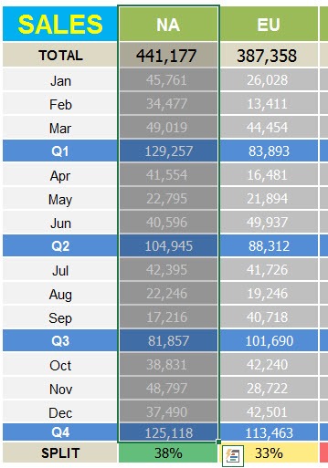
STEP 1: Highlight the range or select the cell that you want the Hyperlink to refer to:
STEP 2: Go to the Name Box on the top left hand corner of the worksheet and enter a name (with no spaces):
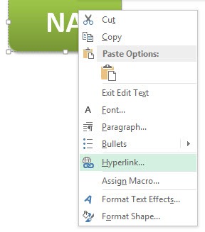
STEP 3: Right Click on an Excel shape and choose Hyperlink:
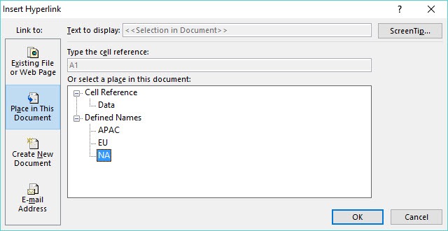
This will open up the Insert Hyperlink dialogue box. Select the Defined Name that you set up in Step 2 and press OK.
STEP 4: Clicking on the Shape will highlight your referenced range.
You can add extra Columns/Rows in your worksheet by selecting the whole Column/Row and pressing the CTRL+ + shortcut.
Clicking on your Hyperlink will follow your referenced range! Cool hey 🙂
John Michaloudis is a former accountant and finance analyst at General Electric, a Microsoft MVP since 2020, an Amazon #1 bestselling author of 4 Microsoft Excel books and teacher of Microsoft Excel & Office over at his flagship Academy Online Course.


