Microsoft Excel‘s VLOOKUP function is a lifesaver for data retrieval, but it’s not immune to glitches. When error messages like #N/A and #VALUE! pop up, it’s your spreadsheet’s way of asking for help. Ignoring these signals can lead to skewed results and costly mistakes in tasks like budgeting and data analysis. In this article, we will cover different ways to fix VLOOKUP error in Excel.
Key Takeaways:
- VLOOKUP errors can derail your data analysis efforts, leading to misinformed decisions.
- #N/A errors often signal missing arguments in your VLOOKUP formula, requiring careful scrutiny and alignment.
- Duplicates in your dataset can confuse VLOOKUP, returning only the first match and potentially distorting your analysis.
- #VALUE! errors typically stem from mismatched value types, highlighting the importance of consistent formatting and data types.
- Utilizing techniques like INDEX-MATCH and error handling functions like IFERROR can enhance VLOOKUP’s accuracy and resilience to errors.
Table of Contents
Introduction to VLOOKUP Glitches
Decoding Common VLOOKUP Mistakes
If you’ve dabbled in the world of Excel, you’ve certainly heard the buzz about VLOOKUP. This powerful function is the go-to tool for searching and retrieving information across your spreadsheet. However, just when you think you’ve mastered it, VLOOKUP might throw a wrench in your plans with pesky error messages like #N/A and #VALUE.
These aren’t just random strings of characters — they’re cries for help from your Excel sheet, signaling that something’s gone awry.
The High Cost of Ignoring Errors
Ignoring errors in your VLOOKUP formulas can be a costly oversight. Whether you’re crunching numbers for a budget, analyzing sales data, or preparing a report, errors can skew your results and lead to misinformed decisions. Beyond the immediate frustration, unresolved errors can ripple through your datasets, creating a domino effect of inaccuracies that undermine the integrity of your work. By not addressing these red flags, you risk presenting flawed data which could have significant consequences, especially in a business setting where strategic decisions hinge on the accuracy of your spreadsheets.
So next time an error pops up, think twice before you brush it off. They’re not just digital hiccups — they’re valuable indicators that something needs your attention. This could mean the difference between a successful project and one that falls short due to preventable inaccuracies.
#N/A Troubles in the Excel Jungle
The Mysterious Case of Missing Arguments
When VLOOKUP flashes the dreaded #N/A, it’s often a sign of a detective story waiting to unfold — the mysterious case of missing arguments. This error tends to surface when one or more pieces of necessary information are absent or incorrectly positioned within the function’s syntax.
Imagine setting off on a treasure hunt but forgetting the map — VLOOKUP experiences a similar dilemma when it lacks the clear directions provided by proper arguments. Each argument in VLOOKUP needs to be meticulously laid out, from the lookup value to the table range and column index number. Failing to line up these elements in their rightful order is like giving your spreadsheet a riddle instead of a command.
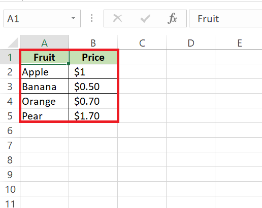
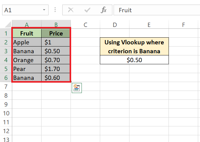
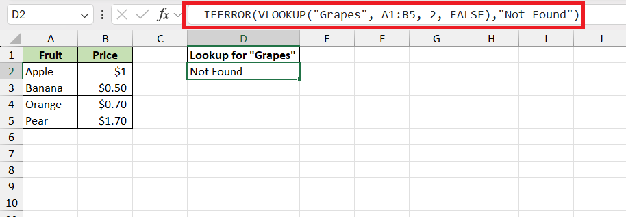
Here’s an example of a dataset and the steps to illustrate a VLOOKUP function with missing arguments in Excel:
STEP 1: Open Excel and input the dataset in cells A1:B5.
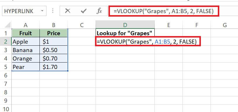
STEP 2: In another cell, say D2, enter the following VLOOKUP function: =VLOOKUP(“Grapes”, A1:B5, 2, FALSE)
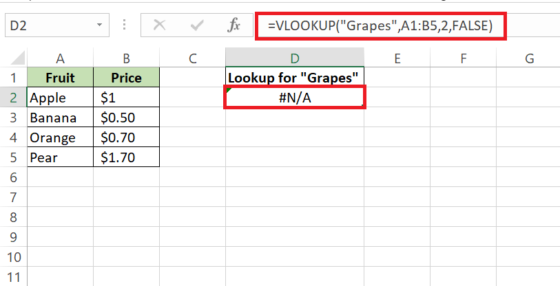
STEP 3: The function searches for “Grapes” in the first column (A1:A5) but won’t find it, resulting in the #N/A error due to the missing lookup value in the dataset.
In this example, the lookup value “Grapes” is missing from the dataset, causing the VLOOKUP function to return the #N/A error. To solve this conundrum, you’ll need to play the role of detective. Double-check each component of your formula.
Is the lookup value specified? Is the table range correctly defined? Did you include the column index number accurately? Are they in the correct sequence? Ensuring each part of the VLOOKUP formula is present and in perfect order is usually the key to making the #N/A error vanish into thin air.
When Duplicates Lead You Astray
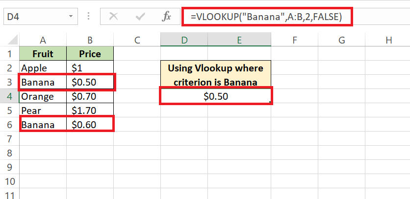
Duplicates in your dataset can take you on a wild goose chase without you even realizing it. In the case of VLOOKUP, if you’re seeking to match a value that appears more than once, you’ll find that VLOOKUP doesn’t play the guessing game; rather, it stops at the first exact match it bumps into. This can cause quite a stir if you’re expecting a different instance of the duplicated value.
For instance, if you’re searching for all the occurrences of a particular item in your inventory list, but VLOOKUP steadfastly returns only the first instance, you might miss out on crucial data points. And if those duplicates are not intentional, they can tarnish your dataset’s quality, possibly leading to erroneous conclusions or misallocated resources.
To navigate through this maze, you need to ensure each entry you wish to look up is distinctive. If not, consider whether the Remove Duplicates tool could help clean up your dataset for a smoother experience. This tool can swiftly eliminate any copycat data, allowing your VLOOKUP function to deliver the single, accurate result you’re after.
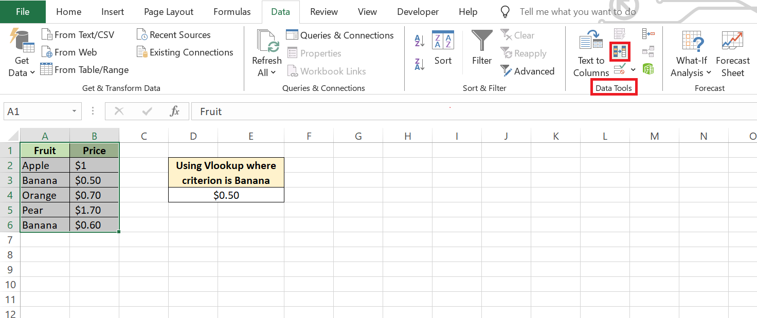
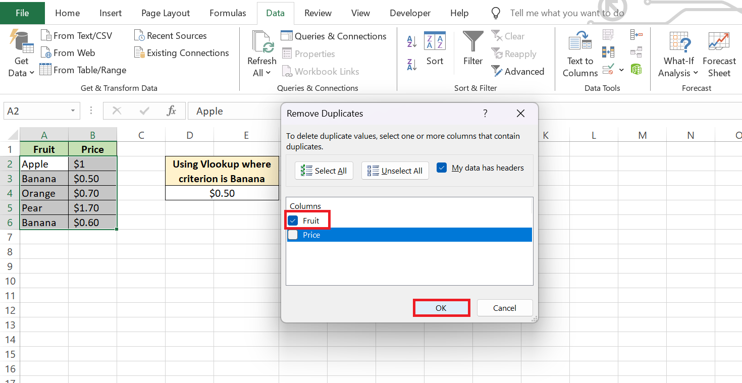
To remove duplicates in this dataset, follow the steps mentioned below:
STEP 1: Select the range containing your dataset.
STEP 2: Go to the “Data” tab.
STEP 3: Click on “Remove Duplicates” in the “Data Tools” group.
STEP 4: Choose the column(s) with potential duplicates (e.g., “Item”) & click “OK”
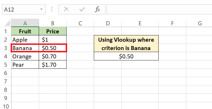
STEP 5: Thus, the duplicate entries are removed.
Dodging the Dreaded #VALUE! Error
Ensuring Your lookup_value is not more than 255 characters.
When encountering a #VALUE! error in VLOOKUP, it’s crucial to ensure that your lookup_value does not exceed 255 characters. Excel has a limitation where the lookup_value argument cannot be longer than 255 characters. If this limit is exceeded, Excel will return a #VALUE! error, indicating that the VLOOKUP operation cannot be completed due to the oversized lookup_value. To avoid this error, ensure that your lookup_value stays within the character limit specified by Excel.
Let’s look at the case below-
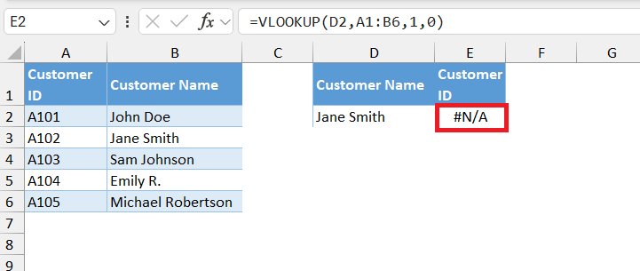
Ensuring Your Lookup Lies Left
Now, you might wonder, “What if the information I need to pull with VLOOKUP is to the left of the column I’m searching?” If you’ve ever been entangled in this conundrum, you’re not alone. VLOOKUP traditionally scans from left to right, and attempting to make it look leftward might feel like teaching an old dog new tricks.
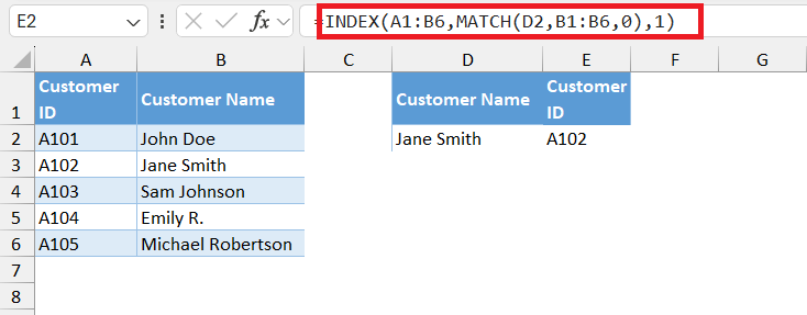
However, contrary to some beliefs, retrieving data to the left of your lookup column isn’t an impossible task. It simply requires swapping out your VLOOKUP hat for an INDEX and MATCH ensemble. This dynamic duo allows you to deftly leap over columns to retrieve your desired value, no matter where it resides within the row.
With INDEX and MATCH, you’re instructing Excel to first find the position of your lookup value using MATCH, then grab the corresponding value that INDEX points out. It’s a game-changer, especially in complex spreadsheets that don’t conform to VLOOKUP’s usual left-to-right comfort zone.
To put this into action, tune into the symphony of INDEX and MATCH working in concert. It may seem intricate at first glance, but once you’ve mastered it, you’ll unlock a level of flexibility that VLOOKUP alone could never achieve.
Pro Tips for Flawless VLOOKUPs
Beware of Extra Spaces and Characters
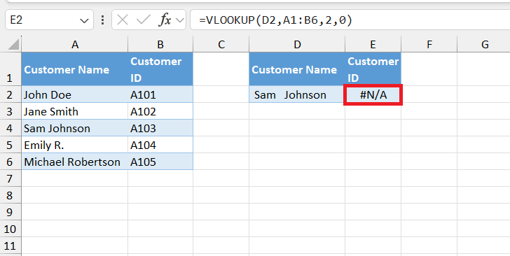
Extra spaces and characters may seem harmless enough, but when it comes to VLOOKUP, they can be the root of a major headache. Just like a tiny pebble in a shoe, these uninvited intruders can throw the whole search off balance, often resulting in the dreaded #N/A error that leaves you scratching your head.
Here’s the thing: VLOOKUP is quite the stickler for exactness. A trailing space or a sneaky non-breaking space (that’s right, they exist!) can sabotage a perfectly good lookup. To excel in the art of VLOOKUP, you need to exterminate these pesky little extras.
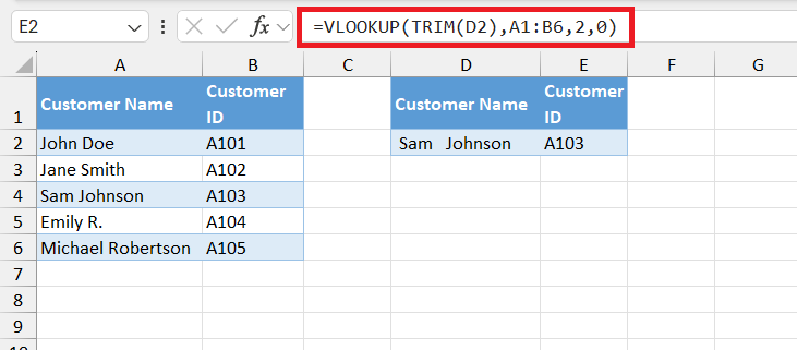
The TRIM function is the hero you need to banish lingering leading and trailing spaces. By wrapping your lookup value with TRIM, you’re essentially giving it a good cleanup, ensuring that no stray spaces are left to confuse your function. Additionally, for those invisible characters that lurk unseen, the CLEAN function is your secret weapon — it removes non-printable characters that may have hitched a ride from other data sources.
Remember, being vigilant about extra spaces and characters is not about nitpicking; it’s about fine-tuning your data for optimal VLOOKUP performance.
The Lifelines for Troubled VLOOKUPs
Using IFERROR and ISNA to Bypass Blunders
When you’re faced with the task of making your Excel sheet error-proof, using IFERROR and ISNA functions is akin to having a trusty shield to bypass blunders gracefully without alarming users with stark error messages.
IFERROR comes to the rescue when you prefer to customize the error message or provide alternative results if VLOOKUP fails. By wrapping your VLOOKUP formula in an IFERROR function, you’re instructing Excel to remain calm and carry on by presenting a friendly message like “Data not found,” or simply a blank cell instead of a jarring #N/A.
FAQ: Excel-lent VLOOKUP Queries Answered
How do I clear a VLOOKUP error?
To clear a VLOOKUP error, first determine the type of error you’re seeing. For #N/A errors, check for correct spelling in your lookup values and ensure there’s an exact match in your table array. For #VALUE! errors, confirm that the value types match, and there are no discrepancies in data format. Use IFERROR function to handle errors gracefully by displaying a custom message or alternative calculation when VLOOKUP fails.
What makes VLOOKUP return an #N/A error?
VLOOKUP returns an #N/A error when it can’t find the lookup value within the specified range. Common culprits include misspellings, incorrect data types, unmatched formats, or lookup values that actually don’t exist in the table array. Always double-check for accuracy and consistency in the data you are searching through.
How do I fix a #VALUE! error in my VLOOKUP formula?
To fix a #VALUE! error in your VLOOKUP formula, ensure that all parameters are correct and properly ordered. Confirm that the lookup value doesn’t exceed 255 characters, and the data types in your lookup column match those in the table array. If necessary, use INDEX-MATCH as an alternative to handle longer lookup values or data types that VLOOKUP struggles with.
How can I ensure VLOOKUP correctly identifies duplicates?
To ensure VLOOKUP correctly identifies duplicates, sort your data to have the preferred record on top, as VLOOKUP will return the first matching value. Alternatively, use a more advanced setup with functions like INDEX, MATCH, and COUNTIF to create a unique identifier for each instance of a duplicated value, allowing you to access all occurrences systematically.
Can formatting affect my VLOOKUP results?
Yes, formatting can significantly impact VLOOKUP results. Number formats mistaken for text, invisible characters, or extra spaces can cause mismatches and errors. Ensure consistency in data format, use the ‘Text to Columns‘ tool or the ‘Convert to Number’ option, and employ functions like TRIM or CLEAN to remove any discrepancies and optimize VLOOKUP’s accuracy.
John Michaloudis is a former accountant and finance analyst at General Electric, a Microsoft MVP since 2020, an Amazon #1 bestselling author of 4 Microsoft Excel books and teacher of Microsoft Excel & Office over at his flagship Academy Online Course.
