What does it do?
A formula that extracts data stored in a Pivot Table
Formula breakdown:
=GETPIVOTDATA(data_field, pivot_table, [field1, item1], [field2,item2],…)
What it means:
=GETPIVOTDATA(return me this value from the Values Area, any cell within the Pivot Table, [and return me the value that pertains to this Field name, and this Field item],…)
The GETPIVOTDATA function in Excel returns data stored in a Pivot Table. So essentially it extracts the Pivot Table data to enable a user to create customized reports.
Think of the Pivot Table like your data source, so anything you see in the Pivot Table report can be extracted with the GETPIVOTDATA function and put into a cell within your worksheet.
The GETPIVOTDATA function becomes powerful when you reference cells to create shell reports, which you can see from the tutorial below.
NB. Only the Fields and Items that are included in the Pivot Table report (Row/Column Labels and Values area) can be used to extract their values.
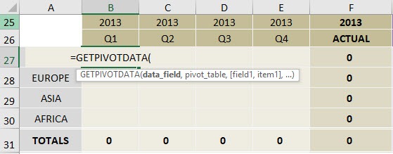
STEP 1: We need to enter the GETPIVOTDATA function:
=GETPIVOTDATA(
STEP 2: The GETPIVOTDATA arguments:
Table of Contents
data_field
What is the value that we want to return?
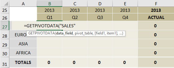
Type in SALES as we want to return the sales value:
=GETPIVOTDATA(“SALES”,
pivot_table
From which pivot table?
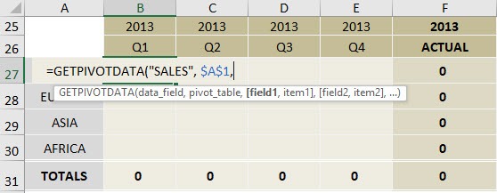
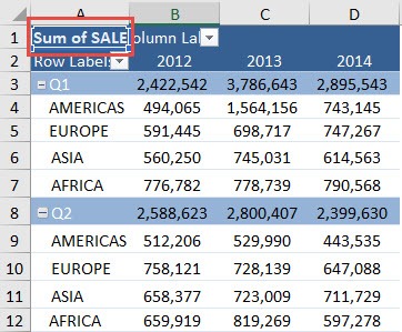
Just reference a cell in the pivot table, let’s type in $A$1
=GETPIVOTDATA(“SALES”, $A$1,
[field1, item1]
What are the fields that would serve as our filtering criteria?
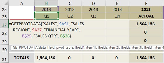
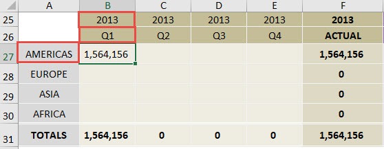
To get our target sales figure, we will need: Sales Region, Financial Year and Sales Quarter. To do this we will need 3 field-item pairs:
=GETPIVOTDATA(“SALES”, $A$1, “SALES REGION”, $A27, “FINANCIAL YEAR”, B$25, “SALES QTR”, B$26)
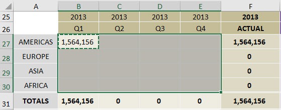
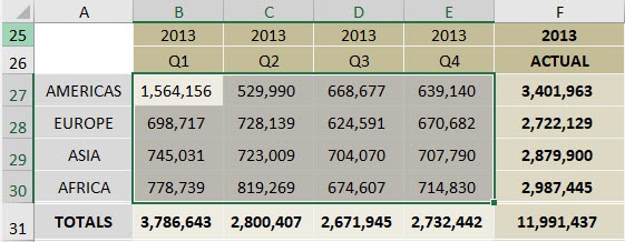
STEP 3: Do the same for the rest of the cells by copying the GETPIVOTDATA formula to the rest of the cells.
Now your new set of data is ready!
John Michaloudis is a former accountant and finance analyst at General Electric, a Microsoft MVP since 2020, an Amazon #1 bestselling author of 4 Microsoft Excel books and teacher of Microsoft Excel & Office over at his flagship Academy Online Course.

