Power Query lets you perform a series of steps to transform your Excel data.
There are times when we want to do things that are not built in the user interface. This is possible with Power Query’s programming language, which is M.
To start off, we will do a simple example of merging the first name and second name into a new column. This is possible with the CONCATENATE formula, however I want to use a simple example for you to get a feel of how to use M in Power Query. Baby steps!
Let’s go through the steps in detail:
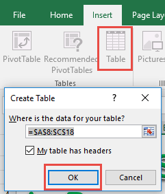
STEP 1: Select your data and turn it into an Excel Table by pressing the shortcut Ctrl + T or by going to Insert > Table
STEP 2: Go to Data > Get & Transform > From Table (Excel 2016) or Power Query > Excel Data > From Table (Excel 2013 & 2010)
Excel 2016:
Excel 2013 & 2010:
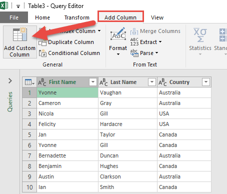
STEP 3: This will open up the Power Query Editor.
Here we will have our first taste of using M!
Go to Add Column > Add Custom Column
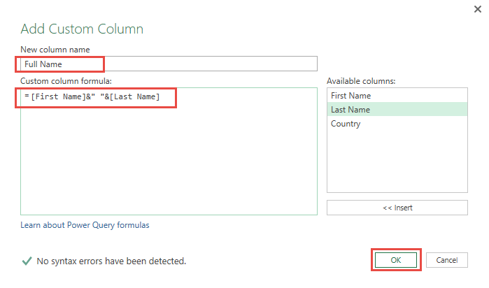
STEP 4: Let us create a simple M expression to combine the First Name and the Last Name.
In the New column name text box, type Full Name
In the Custom column formula, type in: [First Name]&” “&[Last Name]
(You can alternatively double click in the Available columns names to use the column names in the formula)
The Ampersand (&) will combine the values together, then we added a space in the middle with the double quotes ” “
Click OK.
Now you will see your changes take place.
STEP 5: Click Close & Load from the Home tab and this will open up a brand new worksheet in your Excel workbook with the updated values.
Woohoo! You now had your first taste of programming using M! Watch out for future posts as we tackle on more complex formulas!
Bryan
Bryan is a best-selling book author of the 101 Excel Series paperback books.


