How to get Remainder in Excel using MOD Formula
In Excel, it is very easy to divide two numbers.
But how about if you need to get the remainder from a division operation?
For example, divide 13 by 4:
- Divide the two numbers (i.e. 13 / 4)
- Get the quotient (which is 3)
- Multiply it back to the divisor (3 * 4)
- Subtract it from the original number (13 – 12)
- And I have the remainder! (1)
So, 4 goes into 13 three times with a remainder of 1.
Thankfully we can do the above complex and manual calculation with ease using Excel’s MOD formula!
In this tutorial, we will cover the following concepts in detail:
MOD Function – Syntax & Basic Use
What does it do?
Gives you the remainder after dividing one number with another
Formula breakdown:
=MOD(number1, number2)
What it means:
- number1 – A number whose remainder you wish to find.
- number2 – A number to divide with.
So, MOD(13,3) returns 1 as when you divide 13 by 3 will give a quotient of 4 and leaves a remainder of 1.
Let’s look at a few examples to know how to get remainder in Excel using the MOD formula.
Follow the step-by-step tutorial on How to get Remainder in Excel using MOD Formula and make sure to download Excel Workbook to follow along:
STEP 1: We need to enter the MOD function:
=MOD(
STEP 2: The MOD arguments:
Table of Contents
number1
What is the first number that we plan to divide?
Reference the cell that contains the first number:
=MOD(C9,
number2
What is the divisor?
Reference the cell that contains the second number:
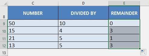
=MOD(C9, D9)
STEP 3: Do the same for the rest of the cells by dragging the MOD formula all the way down using the left mouse button.
Now you are able to get the remainders of all the division operations!
Now that you have learned how to use the MOD function to find the remainder. Let’s move on to some practical uses of this function.
Use MOD function to Highlight Cells
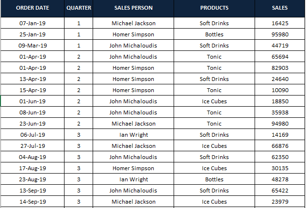
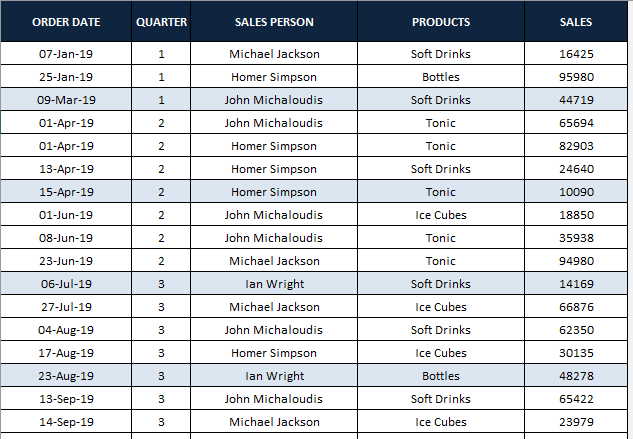
You can use the MOD function to conditionally format the cells. Say, you want to highlight every 4th row in your data.
Let’s see the data table below:
Let’s follow the step-by-step tutorial below to highlight every 4th row of this data table:
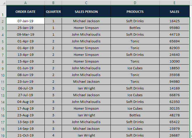
STEP 1: Select the entire data table.
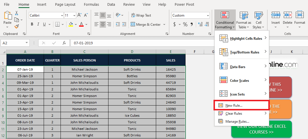
STEP 2: Go to Home > Conditional Formatting > New Rule.
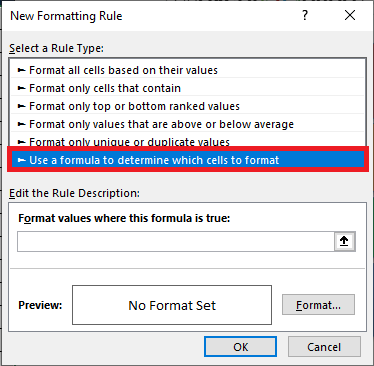
STEP 2: In the New Formatting dialog box, select Use a formula to determine which cells to format from the list.
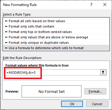
STEP 4: Type the formula
=MOD(ROW(),4)=0
under Format values where this formula is true text box, and then click on Format button to apply custom formatting to these rows.
Using this formula you can add formatting to every 4th row of the data. You can change the number to 2,3,5… as per your need.
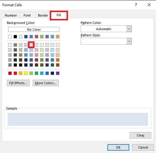
STEP 5: In the Format Cells dialog box, Go to Fill Tab, and select an appropriate color. Click OK.
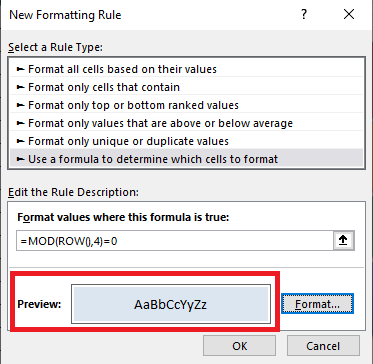
STEP 6: Here you can see a preview of how your formatted data will look like. If you are satisfied with it, click OK.
Your conditionally formatted data table using the MOD formula is now ready!
To highlight, the nth column you can simply replace the ROW formula with the COLUMN formula.
This conditional formatting is dynamic, i.e. once you add or delete more rows the formatting will update automatically.
As you have seen, you can use the MOD function to highlight the nth row or column of your data. You can also use it to sum every nth row/column.
Use MOD function to Calculate cells
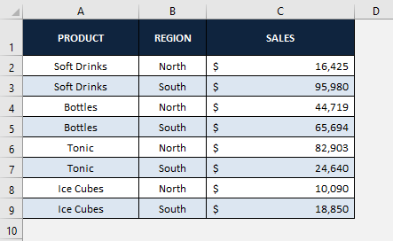
In the data below, you have sales data for different products & different regions.
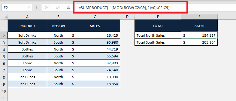
You can use the MOD function, to sum up, every alternate row in the data to get the total sales of the North and South regions separately.
The formula for the sum of every even row (North Region Sales) :
=SUMPRODUCT(- -(MOD(ROW(range),2)=0),range)
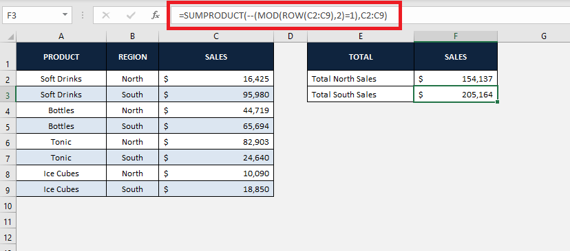
The formula for the sum of every odd row (South Region Sales) :
=SUMPRODUCT(- -(MOD(ROW(range),2)=1),range)
Here,
- The ROW function returns the row number of the cell.
- MOD function when divides an even number leaves remainder as 0 and when divides an odd number leaves remainder as 1.
- Double dashes (- -) outside the MOD function converts the FALSE and TRUE into 0s and 1s.
- Lastly, SUMPRODUCT function multiplies the sum of the product of range containing 0s and 1s and range containing sales amount.
The formula for calculating total sales in North Region i.e., the summation of all even rows (Row 2, Row 4, Row 6 & Row 8) will be:
The formula for calculating total sales in South Region i.e., the summation of all odd rows (Row 3, Row 5, Row 7 & Row 9) will be:
Conclusion
In this tutorial, you have learned not only how to get remainder in Excel but also how to use the MOD function to highlight and calculate cells.
To know more about various functions available in Excel, Click Here!
Further Learning:
- How to Master Excel Formulas – The Ultimate Guide
- 101 Advanced Excel Formulas & Functions Examples
- 3 Quick Ways to Remove Formulas in Excel
Bryan
Bryan is a best-selling book author of the 101 Excel Series paperback books.


