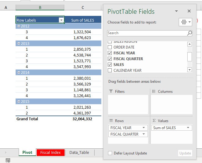
Let us have this setup in our Pivot Table data:
- The Fiscal Year starts in July
- Fiscal Quarters:
- 1st Quarter – July, August, September
- 2nd Quarter – October, November, December
- 3rd Quarter – January, February, March
- 4th Quarter – April, May, June
I will show you how we can set this up!
Exercise Workbook:
We will be using the help of formulas to add two columns to our data source: Fiscal Year and Fiscal Quarter.
Before moving forward let’s get acquainted with the Excel formulas that we will be using here – YEAR(), MONTH() and CHOOSE().
- YEAR() – This formula extracts the YEAR from the date
- MONTH() -This formula extracts the MONTH from the date
- CHOOSE() – This formula extracts a specific value from the list based and the position provided.
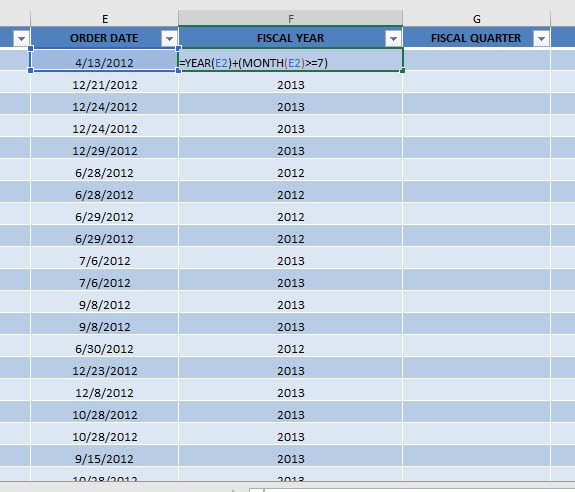
STEP 1: Let us start with the group by Fiscal Years first. Since our fiscal year starts in July, then our formula will be:
=YEAR(E2) + (MONTH(E2) >= 7)
If the month is July or later, then we add one to the year. That will get us the next year as the Fiscal Year.
For example, December 21, 2012, will have the fiscal year of 2013, as it is July or later.
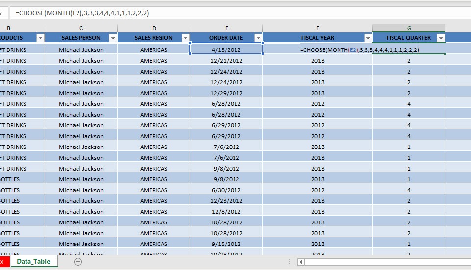
STEP 2: Let us work on the Fiscal Quarter next. Since our first fiscal quarter starts in July, then our formula will be:
=CHOOSE(MONTH(E2),3,3,3,4,4,4,1,1,1,2,2,2)
This formula will simply match the Month number to the sequence of:
- 3rd Quarter – January (3), February (3), March (3)
- 4th Quarter – April (4), May (4), June (4)
- 1st Quarter – July (1), August (1), September (1)
- 2nd Quarter – October (2), November (2), December (2)
For example, December 21, 2012 will have a fiscal quarter of 2 as it will match the last part of the formula:
=CHOOSE(MONTH(E2),3,3,3,4,4,4,1,1,1,2,2,2)
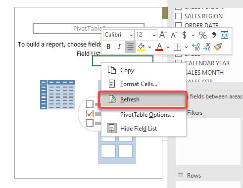
STEP 3: Once the columns are ready, right-click on your Pivot Table and select Refresh
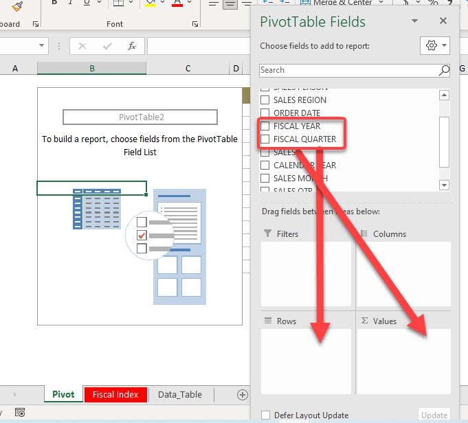
STEP 4: The new Fiscal columns are now there, drag the FISCAL YEAR and FISCAL QUARTER to Rows. Then drag SALES to Values
You now have your Pivot Table ready and group by Fiscal Years and Quarters!
Make sure to download our FREE PDF on the 333 Excel keyboard Shortcuts here:
Bryan
Bryan is a best-selling book author of the 101 Excel Series paperback books.
