Group by Sales Range in Excel Pivot Tables

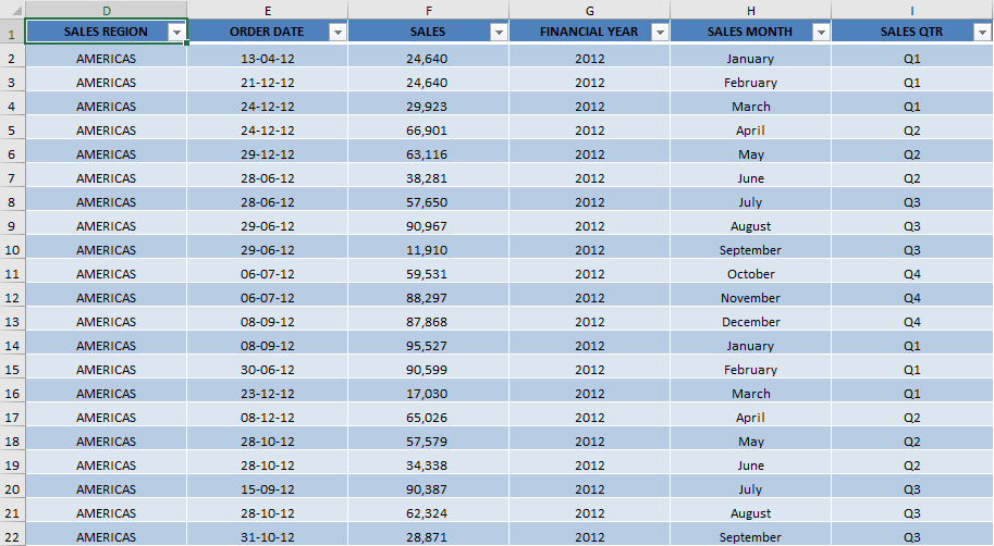
Here is our data table:

We want to use Pivot Tables to create a group by sales ranging between 10,000 to 100,000 and then get a count and sum of sales of these ranges. Following the step-by-step tutorial below this result can easily be achieved:

Don’t forget to download the Exercise Workbook below and follow along with us:

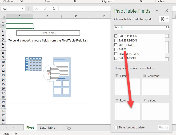
STEP 1: Let us start with an empty Pivot Table. Drag Sales to Rows

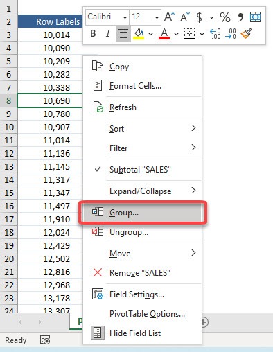
STEP 2: Right-click on any Sales value and select Group

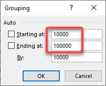
STEP 3: Let us set our group range to 10,000-100,000 with the groupings by 10,000. Click OK.

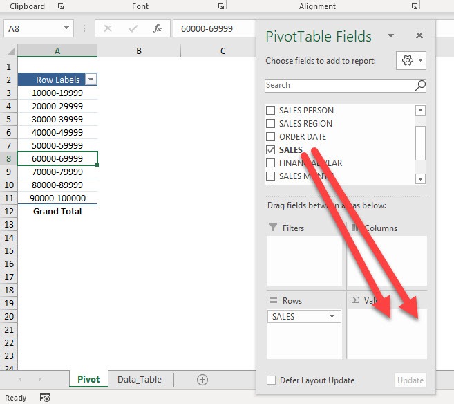
STEP 4: Now drag Sales to Values twice

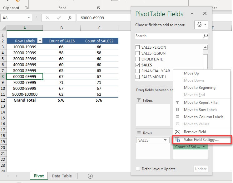
STEP 5: We will get 2 similar columns. We want to have them show the Sum and Count.

Select any one of the columns and pick Value Field Settings

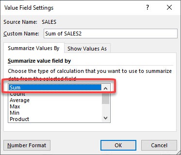
STEP 6: Select Sum and click OK

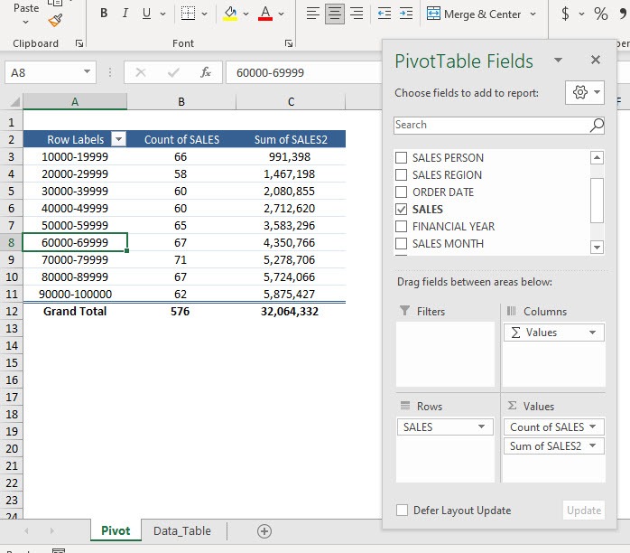
Now you are able to gather data based on the grouped sales figures!

You can use this method to group Pivot Table data by sales range, age, price range or any other numerical data!

Make sure to download our FREE PDF on the 333 Excel keyboard Shortcuts here:

Bryan

Bryan is a best-selling book author of the 101 Excel Series paperback books.

See also  Show/Hide Field Headers in Excel Pivot Tables