Want to know how to Excel Pivot Table group by 15 minutes, 1 hour, or a custom time interval? Keep Reading!
Let’s put yourself in my place for a second.
It was a dark, rainy night in Dublin city and I was working overtime…again!
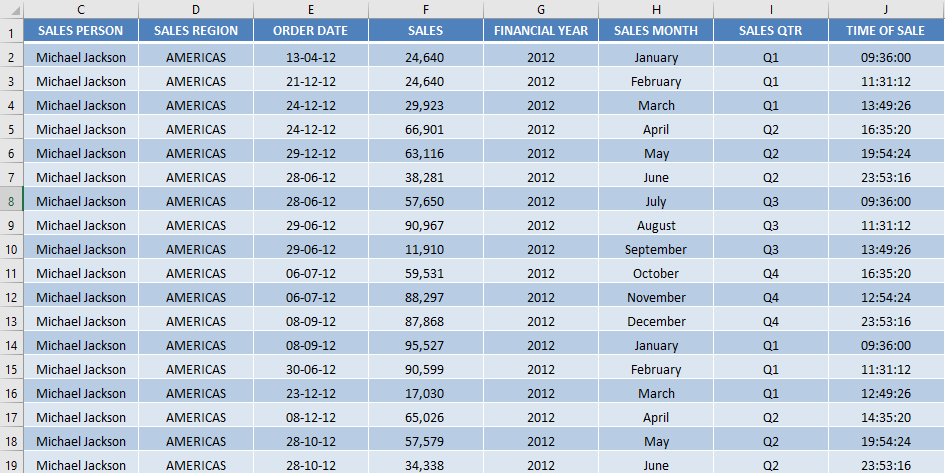
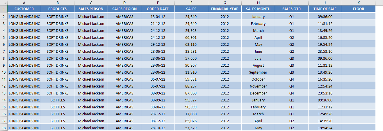
I downloaded a report with lots of transnational data. Time of Sale in one column and Sales in another, among other columns.
I wanted to get the Sales numbers by the hour so that I could understand which part of the day had the best sales and which is the slowest time of the day.
Grouping these would take a ton of effort! Thankfully there is the Pivot Table way, which is quick and reduces the risks of making any errors….and it makes updating the report easy with any new additional data!
In this article, you will be provided a detailed guide on the following:
Let’s look at each one of these methods on How to group time intervals in Excel using a real-life example!
Group by Hour
In the example below, you have Sales data and you want to get the Sales Grouped by Time.
Watch it on YouTube and give it a thumbs-up!
Follow the step-by-step tutorial below on How to group time in Excel and make sure to download the Excel Workbook to follow along:
Download excel workbookGroup-by-Time.xlsx
STEP 1: Insert a new Pivot table by clicking on your data and going to Insert > Pivot Table > New Worksheet or Existing Worksheet
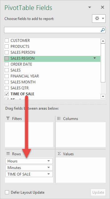
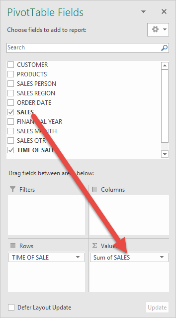
STEP 2: In the ROWS section put in the Time of Sale field.
Notice Excel will automatically Group the Time of Sale field in Excel 2016 (a new feature):
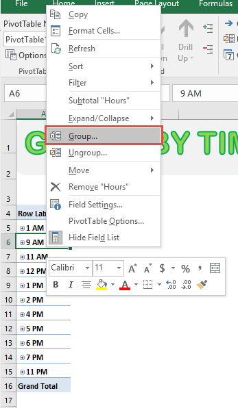
STEP 3: Right-click on any Row item in your Pivot Table and select Group
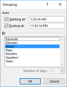
STEP 4: It was able to determine our time range (minimum time and maximum time).
Make sure only Hours is selected (blue highlight).
To create Excel Pivot Table group time by hour, Click OK.
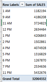
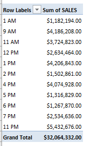
STEP 5: In the VALUES area put in the Sales field. This will get the total of the Sales for each hourly range you have defined:
Now we have our Excel Pivot Table group time by hour, notice that we can improve the formatting:
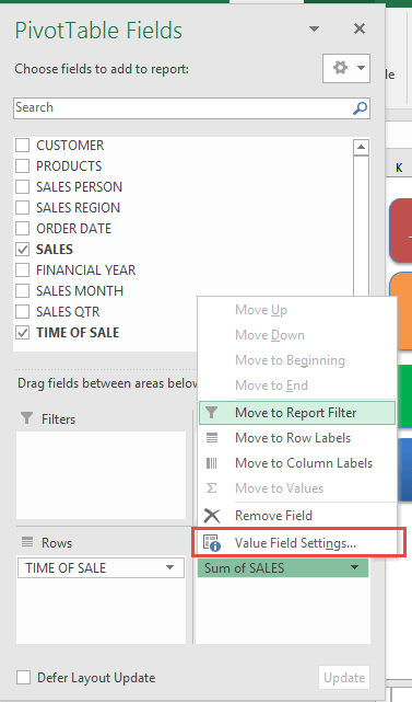
STEP 6: Click the Sum of SALES and select Value Field Settings
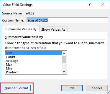
STEP 7: Select Number Format
STEP 8: Select Currency. Click OK.
You now have your total sales for each hourly period!
Extra Tip: You can Right Click on any Sales value in the Pivot Table and select Sort > Largest to Smallest. This will show you the part of the day that has the most sales at the top!
The steps mentioned above can be used to Excel Pivot Table group time by hour.
Group by Custom Time Interval
There might be a time when you want to review the data based on a specific time block instead of a standard 1-hour interval. Like, you want the data to Excel Pivot Table group by 15 minutes or 2 hours or any other custom time interval.
You can easily do that using Excel’s FLOOR function.
Before we learn how to Excel Pivot Table group by 15 minutes, let’s first understand the FLOOR function and its use!
FLOOR Function in Excel can be used to round a number down to the nearest multiple of significance.
The Syntax of the FLOOR function is :
=FLOOR (number, significance)
where
- number – The numeric value you want to round
- significance – The multiple to which you want to round.
Luckily, Excel treats date and time as numbers. The integer portion of the number represents the day and the decimal portion represents the time.
The FLOOR function also accepts an argument in “hh: mm” format and it easily converts them to decimal values. For example, Excel converts 00:15 into 0.0104166666666667, which is the decimal value of 15 minutes, and rounds using that value.
Now, let’s take the same example and create an Excel Pivot Table group by 15 minutes.
STEP 1: Insert a new column named FLOOR.
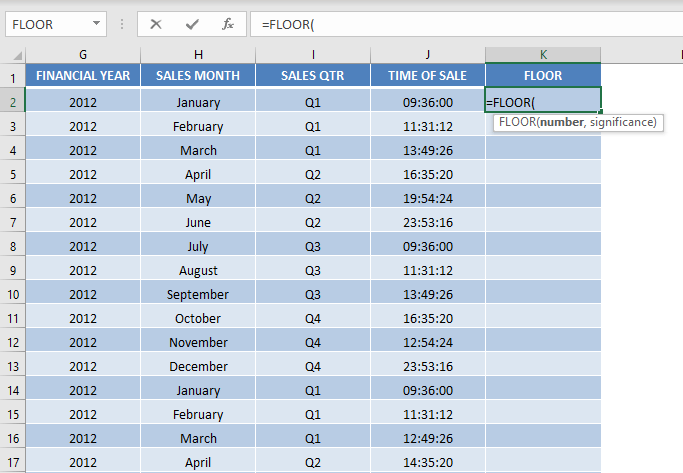
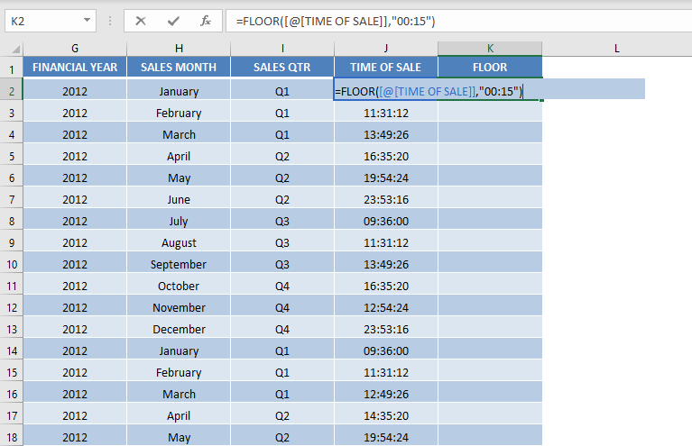
STEP 2: Insert the function FLOOR.
=FLOOR (
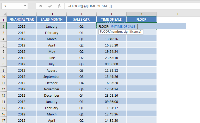
STEP 3: Insert the first argument – Time of Sales.
=FLOOR ([@TIME OF SALES]
STEP 4: Insert the second argument – significance. Here, it is 15 minutes ie 00:15.
=FLOOR ([@TIME OF SALES],”00:15″)
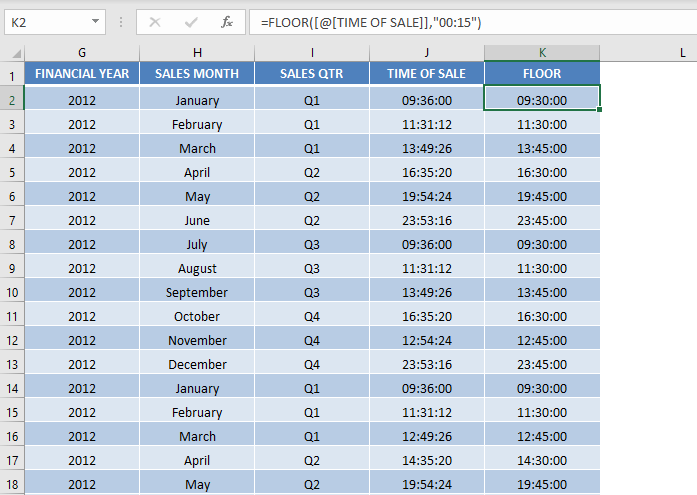
STEP 5: Copy-paste the formula down.
As you can the FLOOR function has rounded the time of sales in intervals of 15 minutes.
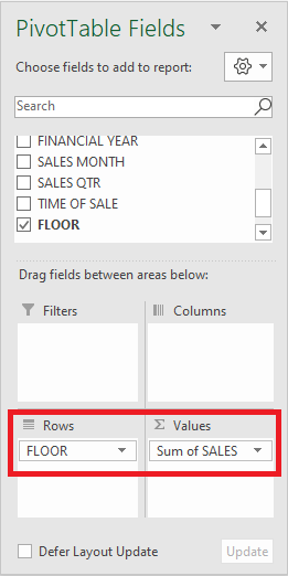
STEP 6: In the PivotTable Fields, drag and drop Time of Sales under Row column and Sales under Values column.
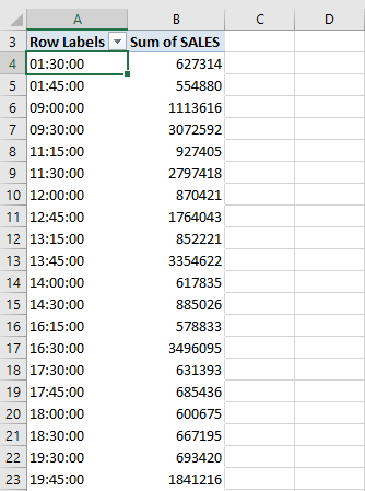
STEP 7: The columns will be displayed in the PivotTable.
This is how you can Excel Pivot Table group by 15 minutes!
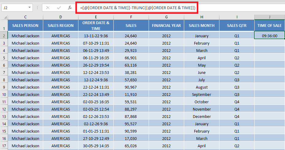
Pro-Tip: In case, you have data containing date and time together, you can easily extract time from that column and then perform the group feature.
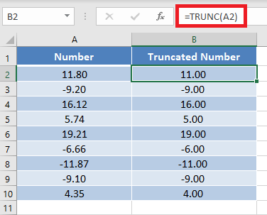
Before we move forward, let’s first understand how to remove decimal from a number in Excel. TRUNC function can be used to truncate a number by removing the decimal portion of a number.
It does not round off the number, it simply truncates the number.
For example, TRUNC(11.8) will return 11, and TRUNC(-9.2) will return -9.
Going back to the previous example!
You can subtract the Date with time from the truncated date and will return only the decimal number. This will extract the time of sales.
This is how you can Pivot Table group by time range like every half hour “0:30” or every five minutes “0:05”.
Conclusion
If you wish you group time by 1-hour interval, you can simply use the group function available in Pivot Table.
But if you want to add a custom time interval like Excel pivot table group by 15 minutes, you can use the floor function to round off the time to a custom interval.
Click here to learn how to Group Dates in Pivot Table!
Further Learning:
- Group by Sales Range in Excel Pivot Tables
- Group Two Excel Pivot Tables Independently
- Group by Text fields in Excel Pivot Tables
Bryan
Bryan is a best-selling book author of the 101 Excel Series paperback books.
