In my previous Group By Month post, we grouped our Sales by each month.
However the cool thing with Excel is that we can take that a step further and customize our grouped date range!
In the example below I show you how to get the Sales Grouped by Custom Dates:
STEP 1: Insert a new Pivot table by clicking on your data and going to Insert > Pivot Table > New Worksheet or Existing Worksheet
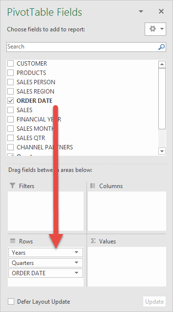
STEP 2: In the ROWS section put in the Order Date field.
Notice that in Excel 2016 (the version that I am using) it will automatically Group the Order Date into Years & Quarters:
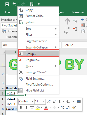
STEP 3: Right click on any row in your Pivot Table and select Group so we can select our Group order that we want:
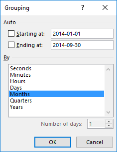
STEP 4: We need to deselect Quarters, Years and make sure only Months are selected (which will be highlighted in blue). This will group our dates by the Months only.
We can now define a custom date range!
For example, we can only show the Sales numbers from January 2014 to September 2014. To do this we need to set the following:
Starting at: 2014-01-01
Ending at: 2014-09-30
Click OK.
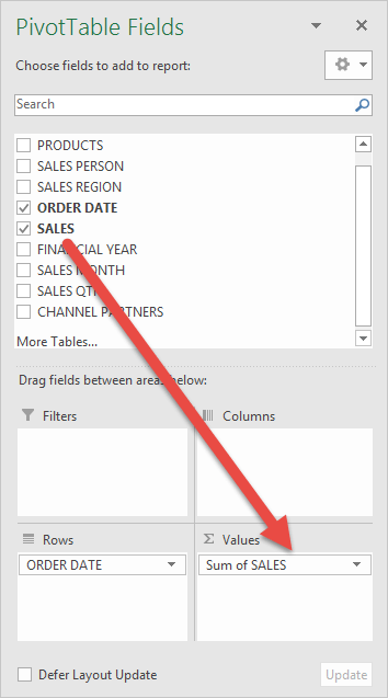
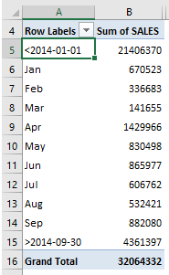
STEP 5: In the VALUES area put in the Sales field. This will show the total of the Sales for each Month:
We can see that everything that does not fall in between January and September is Grouped into its own bucket.
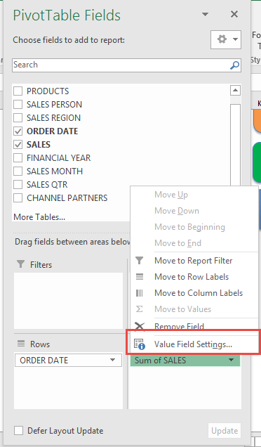
STEP 6: Now we have our sales numbers grouped by Month & Years, notice that we can improve the formatting.
Click the Sum of SALES and select Value Field Settings
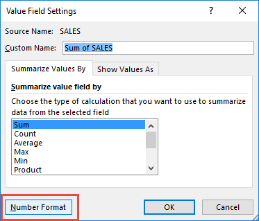
STEP 7: Select Number Format
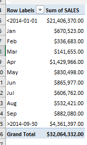
STEP 8: Select Currency. Click OK.
You now have your total sales for each monthly period based on your custom dates! Very Easy!
Bryan
Bryan is a best-selling book author of the 101 Excel Series paperback books.


