Group Sales by Weeks With Excel Pivot Tables

I am sure that your boss has asked you to come up with Total Sales numbers per week at least once in your current role!  If not, he will….very very soon!

Now your data has only sales for each individual day, which makes you scramble to come up with a solution.   How will you be able to group them together and get the sales report your boss needs?

Formulas?  Maybe…well NO!  Too difficult.

Macros?  Don´t know how to code!

Pivot Tables?  HELL YEAH BABY!

Yes, Pivot Tables are quick and reduce the risks of making any errors….ah yeah, I almost forgot…it is also easy to add new data to your sales report!

In the example below I show you how to get the Sales Grouped by Date:

 

STEP 1: Insert a new Pivot table by clicking on your data and going to Insert > Pivot Table > New Worksheet or Existing Worksheet

 

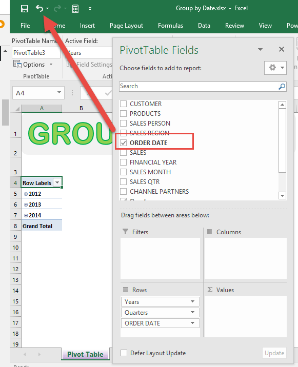
STEP 2: In the ROWS section put in the Order Date field.

Notice that in Excel 2016 it automatically groups dates into Years & Quarters.  We do not need this expansion.

Click the Undo button:

 

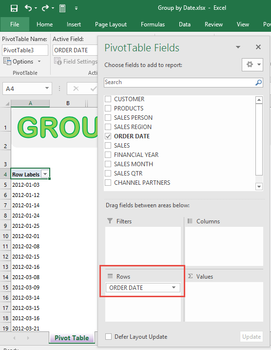
After clicking Undo, you will only have the Order Date in the Rows area:

 

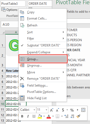
STEP 3: Right click on any date in your Pivot Table and select Group

 

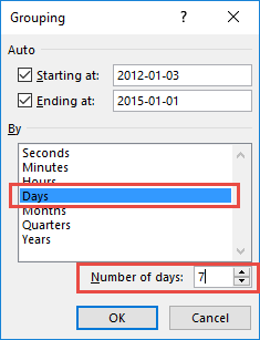
STEP 4: It was able to determine our date range (minimum date and maximum date).

Deselect Months and make sure only Days is selected (depicted by the blue color).

Set the Number of days to 7.

This will group our dates by a weekly range (every 7 days).

Click OK.

 

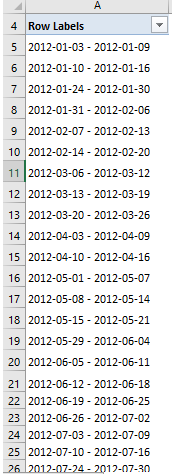
STEP 5: Notice that we have Date Ranges now which are 7 days long each :

 

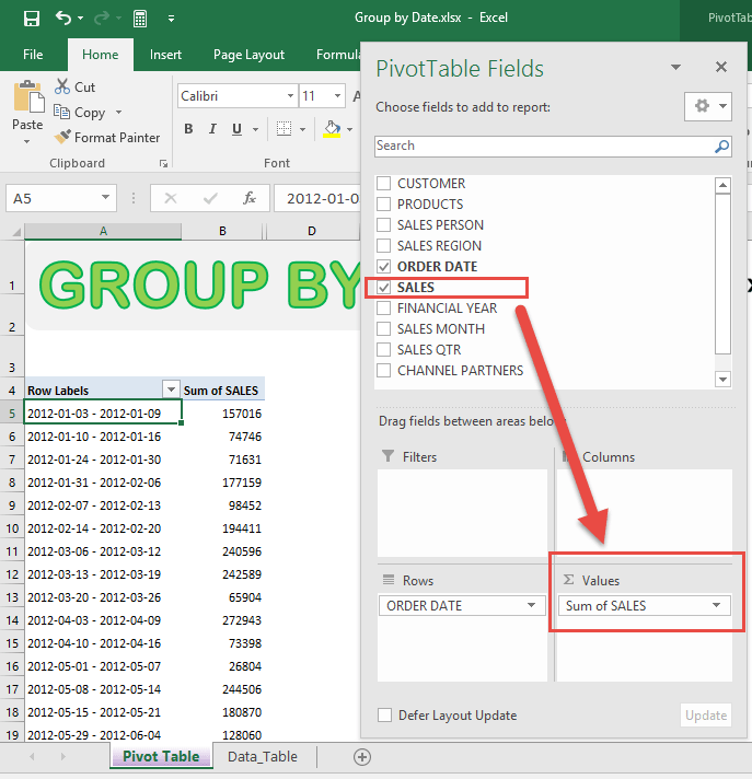
STEP 6: In the VALUES area put in the Sales field.

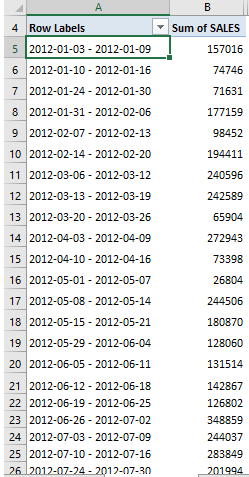
This will get the total of the Sales for each 7-day date range you have defined:

 

You now have your total sales for each 7-day period!  If you like you can insert a Pivot Chart to visually show the data to your miserable boss!