Group By Quarters and Years With Excel Pivot Tables

In the example below I show you how to add quarters to pivot table in Excel:

STEP 1:Insert a new Pivot table by clicking on your data and going to Insert > Pivot Table > New Worksheet or Existing Worksheet

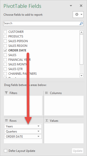
STEP 2: In the ROWS section put in the Order Datefield.

Notice that in Excel 2016 (the version that I am using) it will automatically Group the Order Date into Years & Quarters:

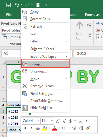
STEP 3:If you do not have Excel 2016, right-click on any Row value in your Pivot Table and select Group 

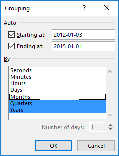
STEP 4:In the Grouping dialogue box,Excelwas able to determine our date range (minimum date and maximum date).

Make sure only Quarters and Years are selected (which will be highlighted in blue).

This will group Excel pivot table quarters. Click OK. 

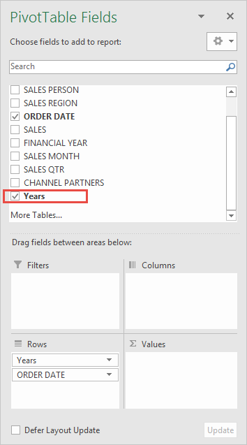
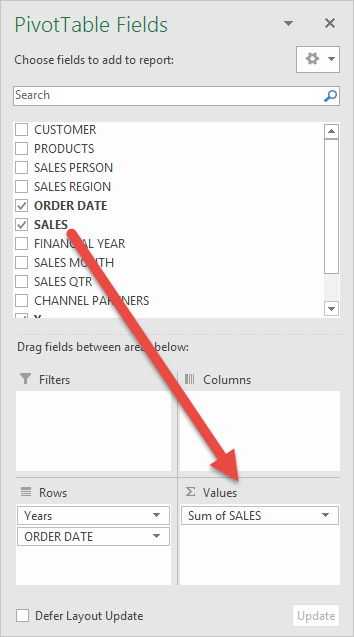
Notice that a Yearsfieldhas been automatically added to our PivotTable Fields List.  This is cool, as we can use this field for further Pivot Table analysis:

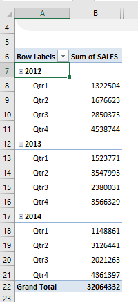
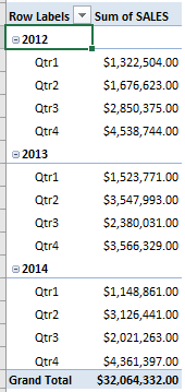
STEP 5: In the VALUES area put in the Salesfield. This will get the total of the Sales for each Quarter-Year date range:

Now we have our sales numbers grouped by Years & Quarters!

Notice that we can improve the formatting:

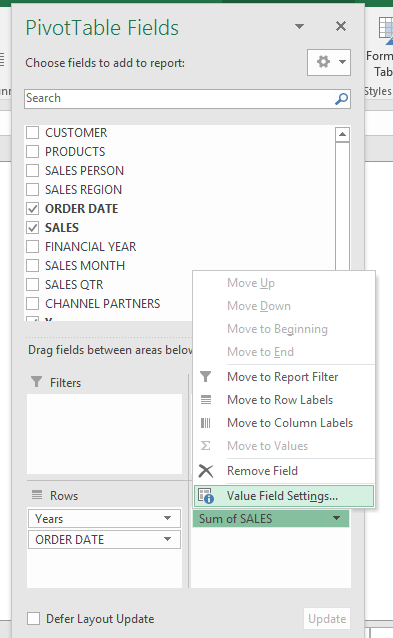
STEP 6: Click the Sum of SALES and select Value Field Settings

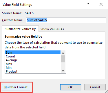
STEP 7: Select Number Format

STEP 8: Select Currency. Click OK.

This is how to add years and quarters to Pivot Table. You now have your total sales for each quarterly period!

Further Learning:

• Group by Fiscal Years & Quarters
• Group by Sales Range in Excel Pivot Tables
• Group by Text fields in Excel Pivot Tables