Power Query lets you perform a series of steps to transform your Excel data.
One of the steps it allows you to take is to group rows and get the counts of each group very easily.
Download excel workbookGroup-By-Count.xlsx
Let’s go through the steps in detail:
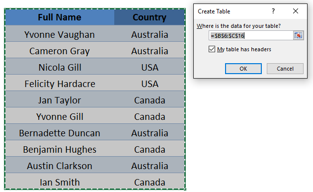
STEP 1: Select your data and turn it into an Excel Table by pressing the shortcut Ctrl + T or by going to Insert > Table
STEP 2: Go to Data > Get & Transform > From Table (Excel 2016) or Power Query > Excel Data > From Table (Excel 2013 & 2010)
Excel 2016:
Excel 2013 & 2010:
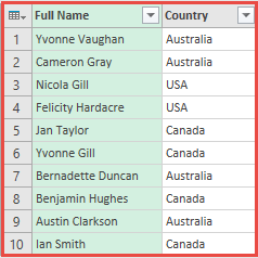
STEP 3: This will open up the Power Query Editor.
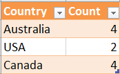
We want to group this data by Country and show how many times each Country appeared in the table. (i.e. Australia appears 4 times in this table)
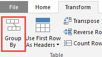
STEP 4: Within here you need to select Transform > Group By
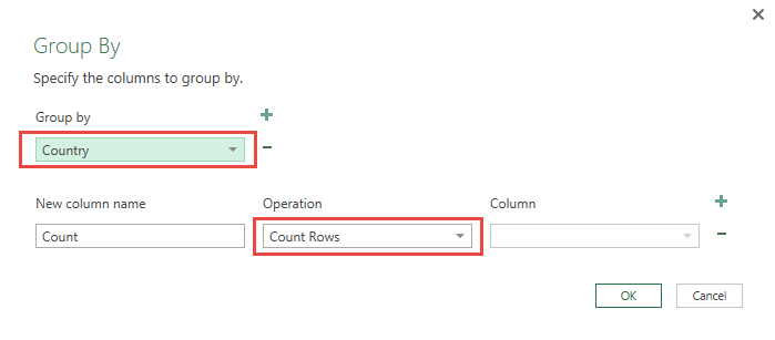
STEP 5: Make sure to select Country for Group By, and select Count Rows for the Operation.
This will group your table by Country value, and count the number of occurrences of each country.
For example, the country of Australia appears 4 times in our table.
STEP 6: Now you will see your changes take place. And the data has now been grouped together.
STEP 7: Click Close & Load from the Home tab and this will open up a brand new worksheet in your Excel workbook with the new data.
You now have your new table with the counts of each country.
Bryan
Bryan is a best-selling book author of the 101 Excel Series paperback books.

