Ever faced a situation when you have asked to prepare a Weekly sales report?
Creating a Weekly report is super easy in Excel. There are several options in Excel that you can perform to get a Weekly Report:
Let’s look at these methods in detail below.
Follow the step-by-step tutorial below and make sure to download the Excel workbook to follow along:
Using WEEKNUM formula
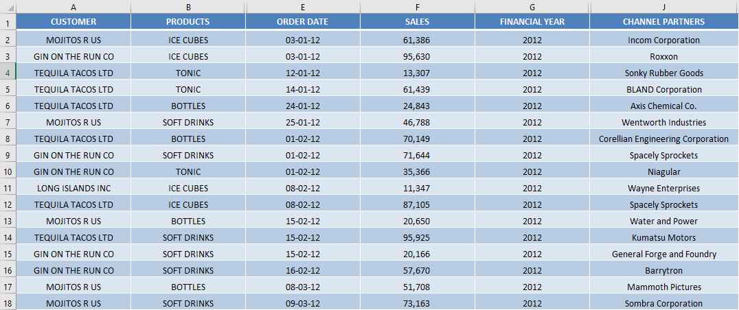
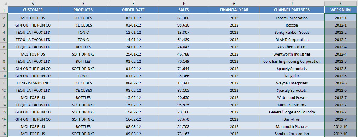
In the screenshot below, you have sales data for a company for which you need to create a weekly report.
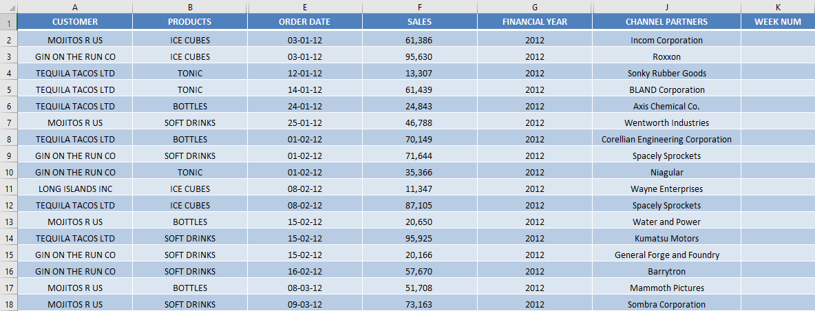
STEP 1: Create a new helper column that will provide the week numbers for the dates.
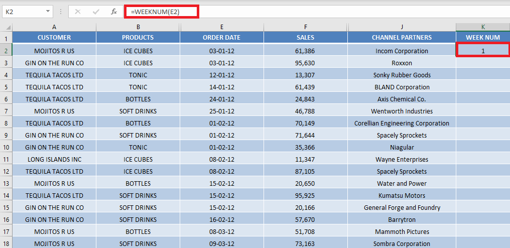
STEP 2: Use the formula – WEEKNUM. It will simply return the week number of a specified date. By default, Excel will consider that the week will begin from Sunday.
Type the formula: =WEEKNUM(E2)
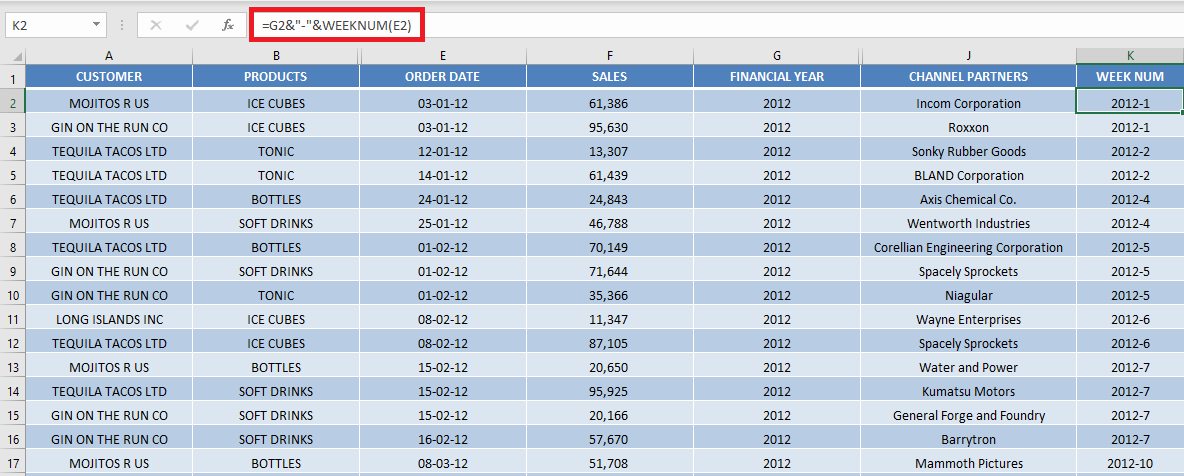
STEP 3: This report contains multiple years. Week number should be combined with the year to provide accurate results.
To combine year and week num, use the formula: =G2&”-“&WEEKNUM(E2,1)
STEP 4: Copy-paste the formula below.
STEP 5: Go to Insert > PivotTable.
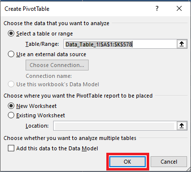
STEP 6: In the Create PivotTable dialog box, Click OK.
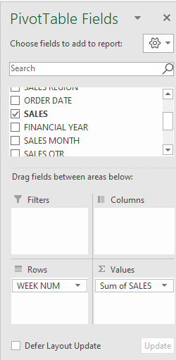
STEP 7: Drag and drop Week Num in the Row field and Sales in the Values field.
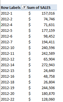
This will provide you with a Weekly Sales Report in Excel using the Weeknum formula.
You can also use the group selection feature in Pivot Tables to Excel group by week. Let’s dive into this method and see how it works.
Using Group Selection
Last time we learned about Excel Group by Week using Pivot Tables. But what if your boss wanted all of the weeks to start on a Monday?
You would be scrambling to find a way to ensure all weeks start on a Monday!
But here’s the thing, setting it to start on Mondays is very easy!
In these examples below I show you how to Excel group by week starting from any day you choose.
EXAMPLE 1:
Follow the step-by-step tutorial below on How to group dates into weeks in Excel:
STEP 1: Insert a new Pivot table by clicking on your data and going to Insert > Pivot Table > New Worksheet or Existing Worksheet
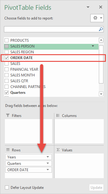
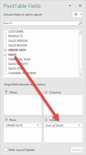
STEP 2: In the ROWS section put in the Order Date field.
Notice that in Excel 2016 it automatically groups dates into Years & Quarters.
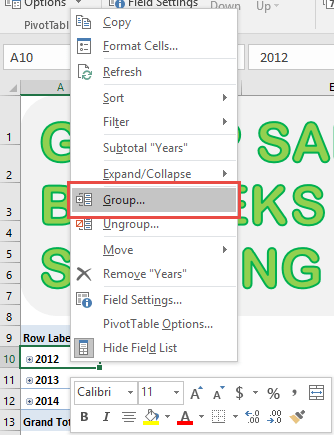
STEP 3: Right-click on any entry in your Pivot Table Row Labels and select Group
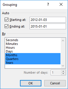
STEP 4: Notice that it was able to determine our minimum and maximum dates. However, we need our weeks to start on a Monday.
Our starting date is January 3, 2012. Let us have a quick check-in our calendar:
We can see that the nearest Monday before that date, is January 2, 2012.
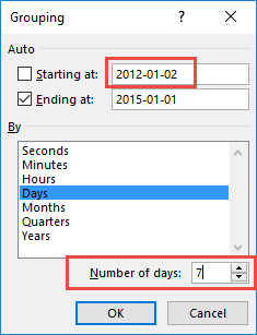
Deselect Months, Quarters, and Years and make sure only Days is selected (depicted by the blue color).
Set the Number of days to 7.
Set the Start Date as 2012-01-02.
This will Excel group by week (every 7 days starting on a Monday).
Click OK.
STEP 5: In the VALUES area put in the Sales field.
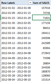
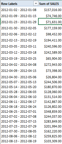
This will get the total of the Sales for each 7-day date range you have defined:
This will create an Excel pivot table group by week!
STEP 6: We can now format our Sales numbers into something more presentable.
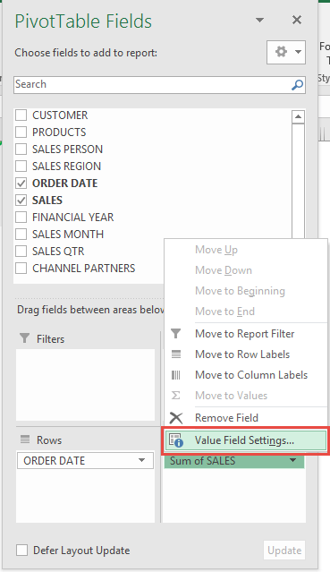
Click the Sum of SALES and select Value Field Settings.
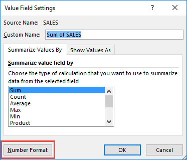
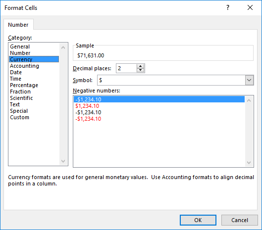
STEP 7: Select Number Format
STEP 8: Select Currency. Click OK.
You now have your total sales for each 7-day period starting on Mondays!
Let’s look at another example in which you can Excel group by week starting from a Sunday!
EXAMPLE 2:
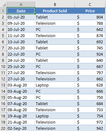
In the example below, there are sales data including sales date, product name, and price sold.
STEP 1: Go to Insert > PivotTable.
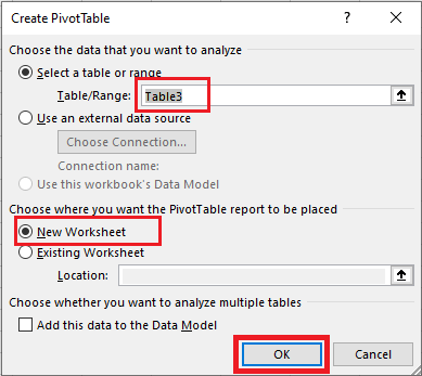
STEP 2: In the Create PivotTable dialog box, select the table range and new worksheet option, and click OK.
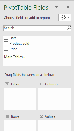
STEP 3: A PivotTable structure will be created in a new worksheet and you can use the PivotTable fields to create a report.
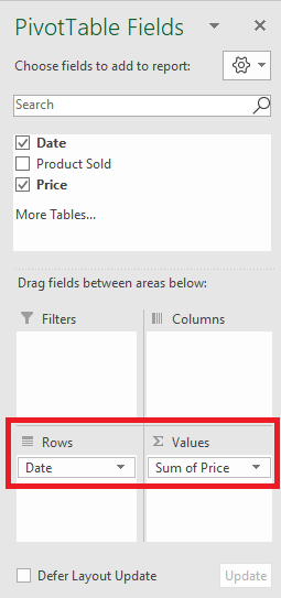
STEP 4: Drag and drop Date in the Row field and Price in the Values field.
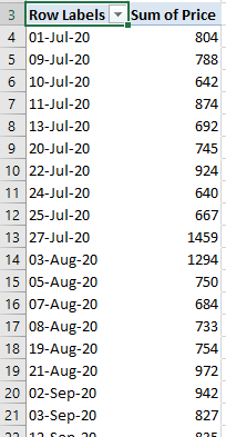
This is how the PivotTable will look like:
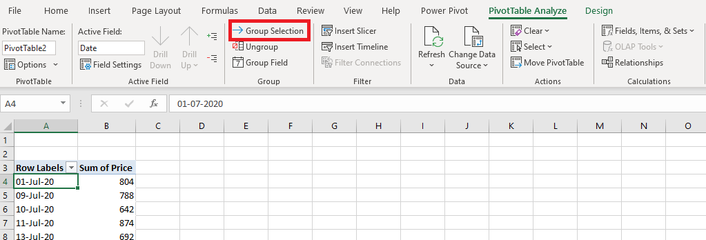
STEP 5: Select any cell in the Date column and then Go to PivotTable Analyze > Group Selection.
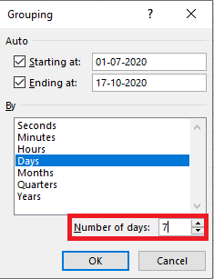
STEP 6: In the Grouping dialog box, select Days (deselect any other option highlighted) and type 7 in the number of days section.
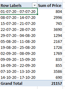
This will group the Pivot Table by a 7-days period.
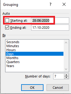
STEP 7: Type the first Sunday in the given range i.e. 28-06-2020 in this Starting at section.
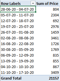
Your weekly sales report starting from a Sunday is now ready!
Similarly, you can also group dates by month, year, hour, second, etc.
Ungroup Data
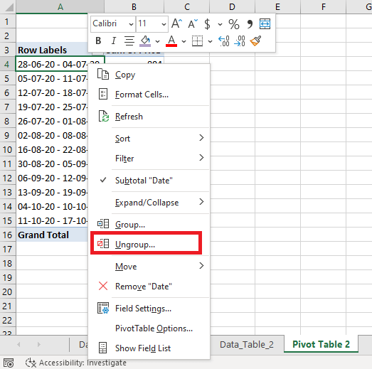
Also, you can easily remove these groups created by following one of the two methods mentioned below:
- Method 1: Right-click on the date column and click Ungroup.
- Method 2: Go to PivotTable Analyze and click on Ungroup.
Conclusion
You can easily analyze data by week, month, year, days, hour, etc., and find trends using this either WEEKNUM formula or Excel group by week feature in Pivot Table.
These are fairly simple and super quick methods to group dates.
Did you know there are many creative ways of doing grouping in Excel Pivot Tables? Click here to learn all about it here!
Further Learning:
- Group by Fiscal Years & Quarters
- Group by Text fields in Excel Pivot Tables
- Errors when grouping by dates
Bryan
Bryan is a best-selling book author of the 101 Excel Series paperback books.
