A Pivot Table has a large amount of data that can be much easier read by highlighting the specific values that need to be viewed. One of the most common ways of highlighting values in pivot tables is by using conditional formatting.
Adding conditional formatting to Pivot Tables can brighten up the data and make it easier to analyze and interpret.
Let us see how one can highlight cell rules based on date labels in a pivot table.
Download this Excel Workbook and follow the step-by-step tutorial below:
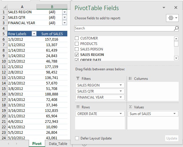
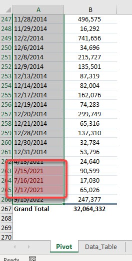
This is our current Pivot Table setup. We want to highlight all of the dates of the current month (July 2021) in our Row Labels.
Example 1:
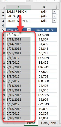
STEP 1: Highlight all the date labels by clicking above the cell
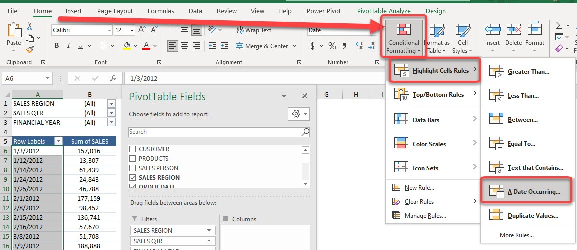
STEP 2: Go to Home > Conditional Formatting > Highlight Cells Rules > A Date Occuring
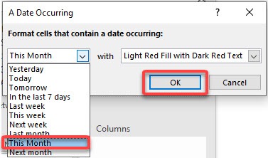
STEP 3: Select This Month and select OK. You can select any color that you wish.
The dates for this month are now highlighted! You can do the same for Column Labels as well.
The best part is this is dynamic, if you open this workbook again next month, the highlighted date values will be for the next month instead!
Example 2:
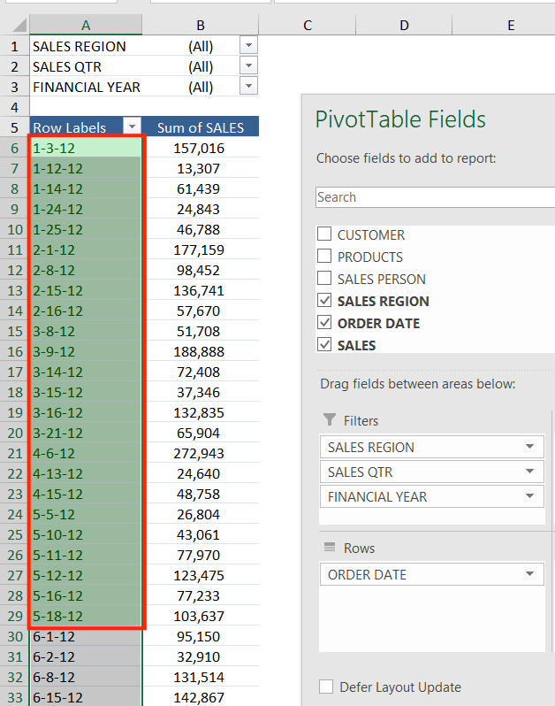
Further elaborating on this, we can even highlight a certain range of dates that we want to focus on. This can be achieved through the following steps:
STEP 1: Highlight all the date labels by clicking above the cell
STEP 2: Go to Home > Conditional Formatting > Highlight Cells Rules > Between…
STEP 3:Enter the range of dates that you want to be highlighted and select a style in which you want the cells to be highlighted.
The dates that lie within this range are now highlighted!
This is how you can highlight cell rules based on date labels by using conditional formatting in Pivot Table!
Make sure to download our FREE PDF on the 333 Excel keyboard Shortcuts here:
Bryan
Bryan is a best-selling book author of the 101 Excel Series paperback books.
