You can use conditional formatting with Excel Pivot Tables to highlight cell rules based on text labels. Let me show you how easy this is with the help of examples.
Download this Excel Workbook and follow the step-by-step tutorial below:
Example 1:
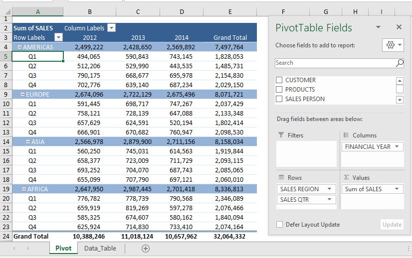
This is our current Pivot Table setup. We want to highlight all of the Q1 text in our Row Labels.
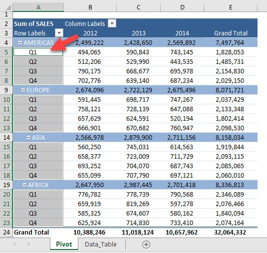
STEP 1: Highlight all the quarter text by clicking above the cell
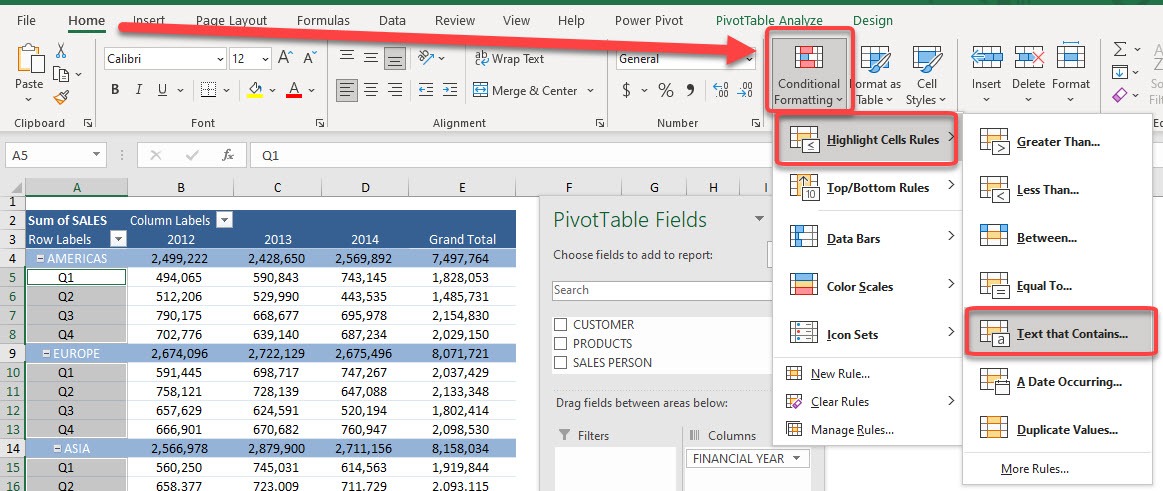
STEP 2: Go to Home > Conditional Formatting > Highlight Cells Rules > Text that Contains
STEP 3: Type in Q1 and select OK. You can select any color that you wish.
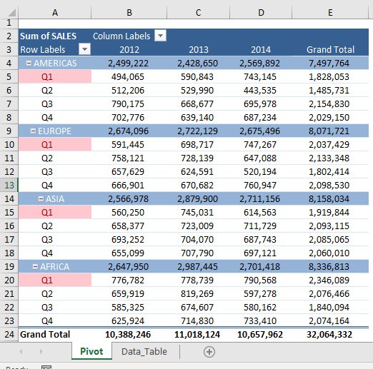
The Q1 text is now highlighted! You can do the same for Column Labels as well
Example 2:
In this example, we want to highlight all quarters except Q4 in red.
STEP 1: Highlight all the quarter text by clicking above the cell
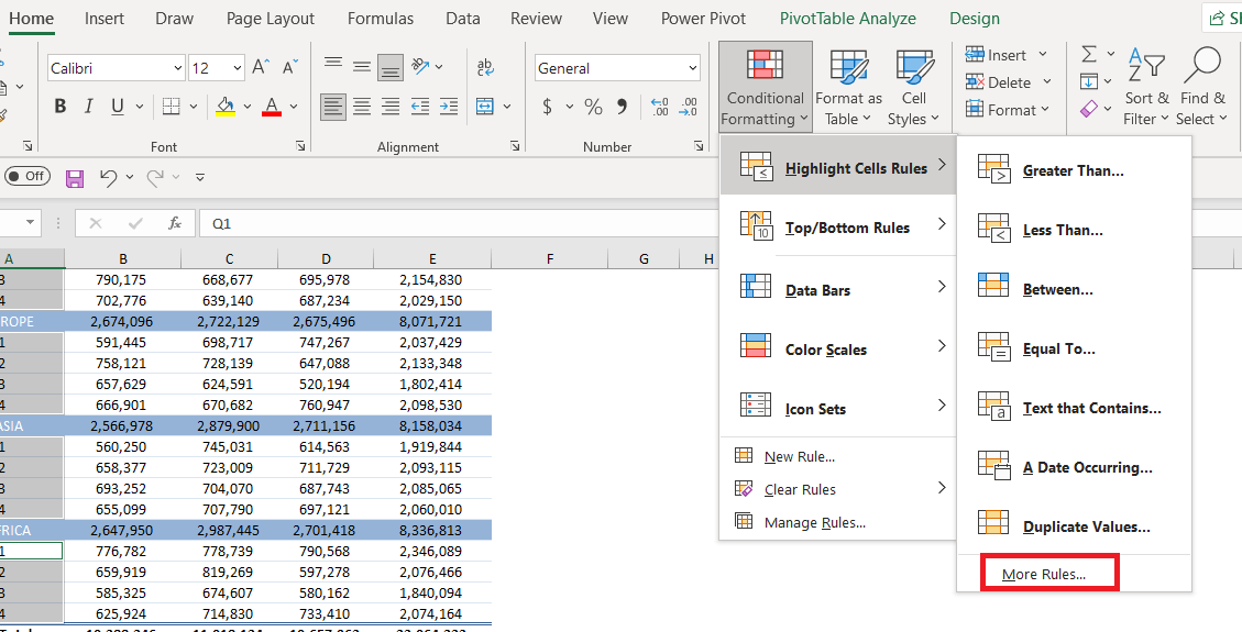
STEP 2: Go to Home > Conditional Formatting > Highlight Cells Rules > More Rules
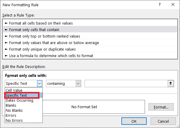
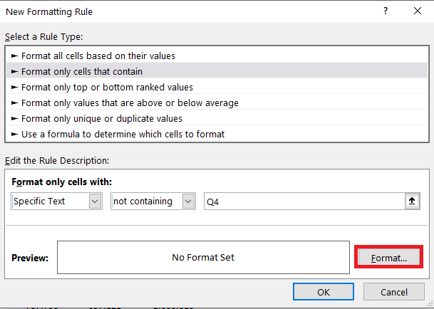
STEP 3: In the New Formatting Rule dialog box, select Specific Text from the first dropdown.
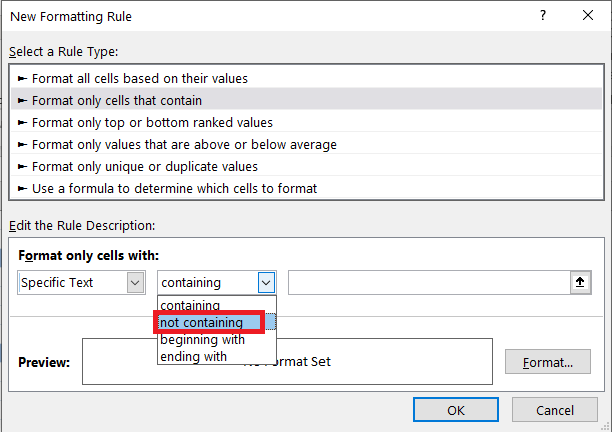
STEP 4: Select not containing from the second dropdown.
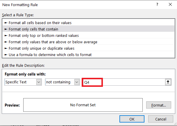
STEP 5: Type Q4 in the space shown below.
STEP 6: Click on the Format… button.
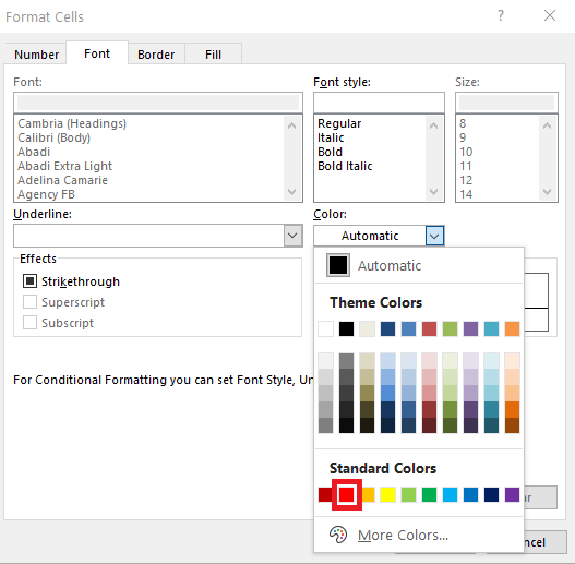
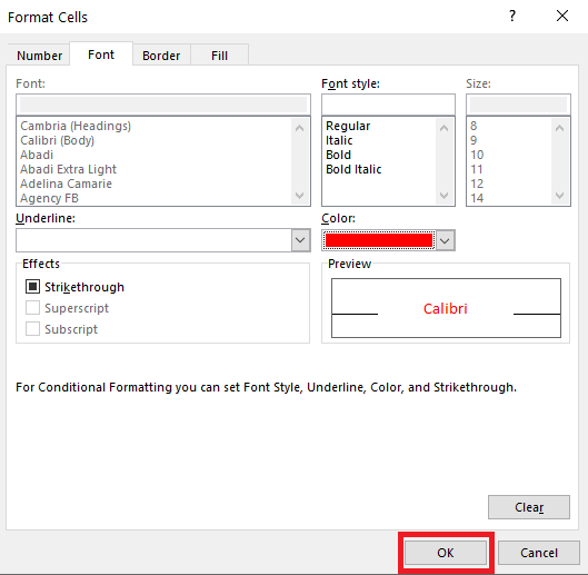
STEP 7: In the Format Cell dialog box, select the red color.
STEP 8: Click OK.
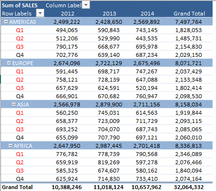
This is what the data will look like:
All quarters except Q4 have been highlighted in red!
Make sure to download our FREE PDF on the 333 Excel keyboard Shortcuts here:
Bryan
Bryan is a best-selling book author of the 101 Excel Series paperback books.
