In Excel, you are usually working with a large dataset, and encountering a duplicate value is really common. It may lead to incorrect formulas or calculations making the data inconsistent or inaccurate.
You can easily spot and highlight duplicates in Excel using a really versatile feature – Conditionally Formatting. If you are not unfamiliar with this feature, it would be a good idea to go through it before we proceed. Click here to learn all about Conditional Formatting.
In this article, you will be covering the following topics in detail –
- Highlight Duplicates Values using Conditional Formatting
- Highlight Duplicates expect 1st Occurence
- Highlight Duplicate Rows
- Remove Duplicates
- Put Unique Values in Another column
Let’s look at each of these topics one by one!
Download the Excel Workbook below to follow along and understand how to highlight duplicates in Excel –
download excel workbookHighlight-Duplicates-in-Excel.xlsx
Highlight Duplicates using Conditional Formatting
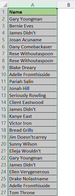
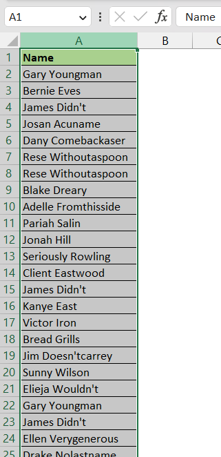
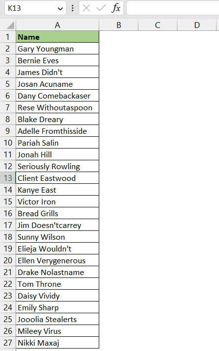
There is an in-built feature in conditional formatting that can be used to highlight duplicates. In this example, you have a list of employee names in Column A and you want to highlight the duplicate ones in red. Follow the steps below to apply it –
STEP 1: Select the range that contains duplicate values.
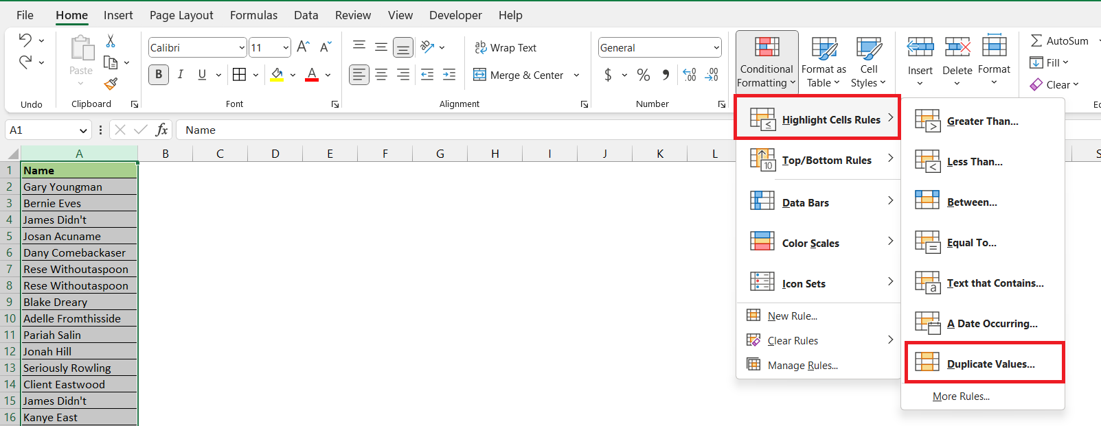
STEP 2: Go to the Home Tab > Click on Conditional Formatting in the Styles group.
STEP 3: Select Highlight Cells Rules > Duplicate Values.
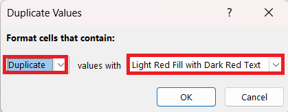
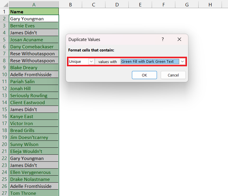
STEP 4: In the Duplicate Values dialog box, select Duplicate and then the formatting that you want to apply. In this example, let’s select Light Red Fill with Dark Red Text.
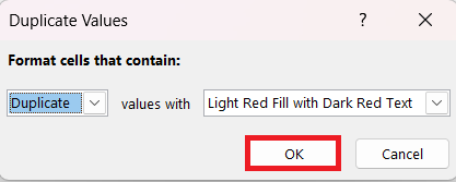
STEP 5: Click OK.
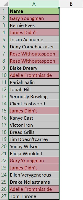
You can see that all the duplicate values in the range will be highlighted based on the formatting that you have selected.
Pro Tip – In the dropdown, you can select Unique and all the unique values will be highlighted in the range.
Highlight Duplicates expect 1st Occurence
In the previous example, what if you want to highlight all duplicates except the first occurrence? Excel has a way around that – you need to use a combination of the COUNTIF function and conditional formatting.
Follow the steps below –
STEP 1: Select the range that contains duplicate values.
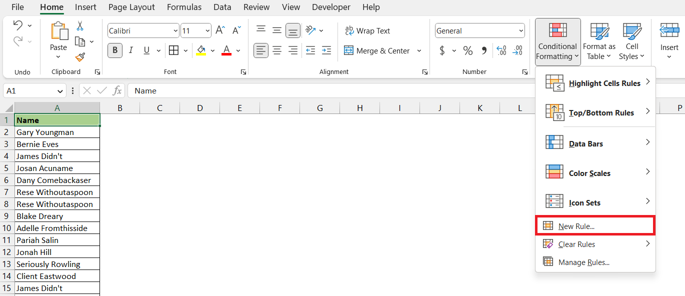
STEP 2: Go to the Home Tab > Click on Conditional Formatting in the Styles group.
STEP 3: Go to New Rule.
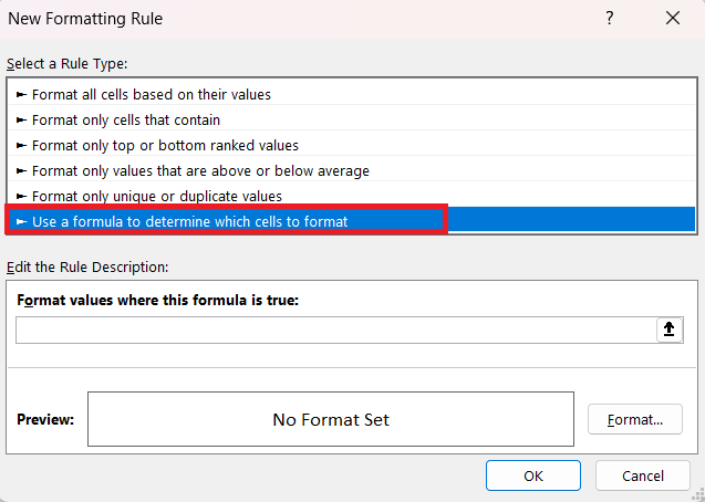
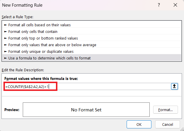
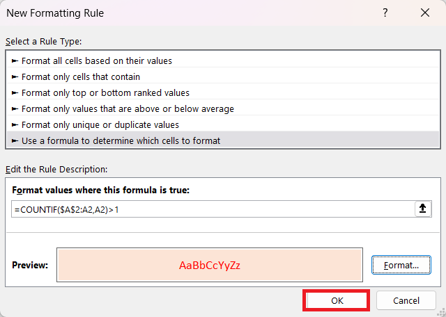
STEP 4: In the New Formatting Rule dialog box, select Use a formula to determine which cells to format.
STEP 5: Enter the following formula in the Edit Rule Description section –
=COUNTIF($A$2:A2,A2)>1
Here, we are using a mixed reference range ($A$2:A2) -where the first cell in the reference is locked ($A$2) and the second range is left relative (A2). As you copy the formula down, the range will keep accommodating a new row. So, the COUNTIF formula will check values from the first location ($A$2) till the current location (say, A5) and will avoid the values below (from A6 to A32).
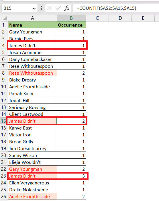
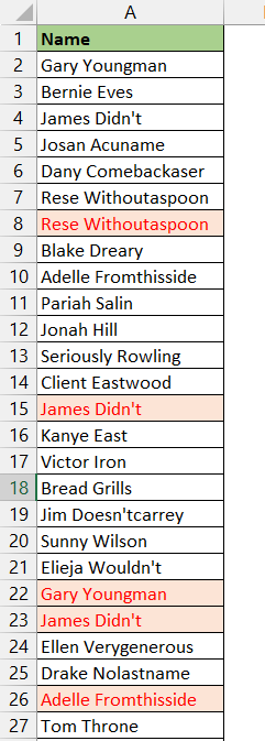
For example, when COUNTIF is running the formula in cell A15, it will count the occurrence of “James Didn’t” from A2 to A15 and will display the result i.e. 2. It will not take into consideration the names mentioned in the range A16 to A32.
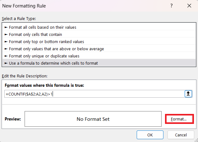
STEP 6: Click on the Format button.
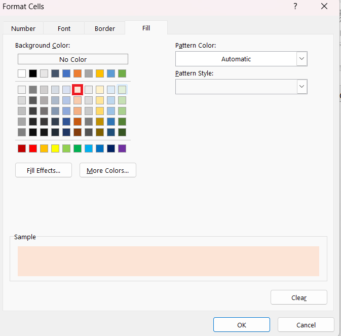
STEP 7: Go to the Fill tab and select a light red color.
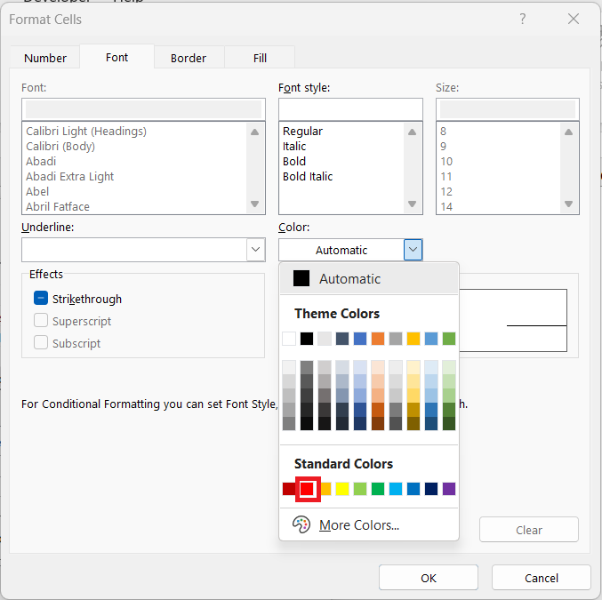
STEP 8: Go to the Font tab and select a red color.
STEP 8: Double-check the formatting for duplicates in the Preview section and press OK.
All the duplicates except the first occurrence has been highlighted in red font and light red fill.
Highlight Duplicate Rows
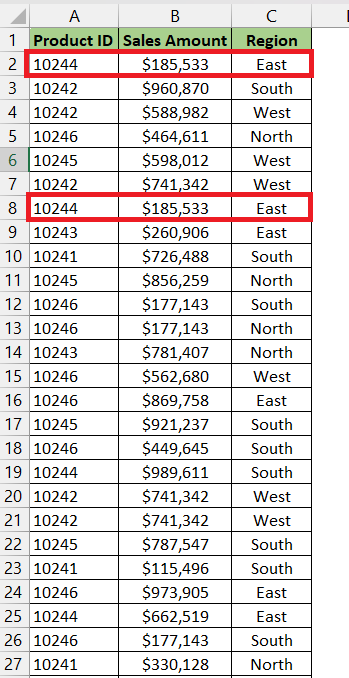
Until now, we analyzed and highlighted duplicates based on values entered in a cell. The in-built feature of conditional formatting looks for value cell by cell only. Now, we want to look at the entire row’s content and then check for duplicates.
In this example, we want to highlight a row only when values in all three columns are the same for any 2 rows.
We will be using the CONCAT function to create a helper column that will help us in highlighting duplicate rows. Follow the steps below to highlight duplicate rows –
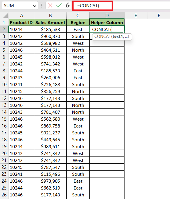
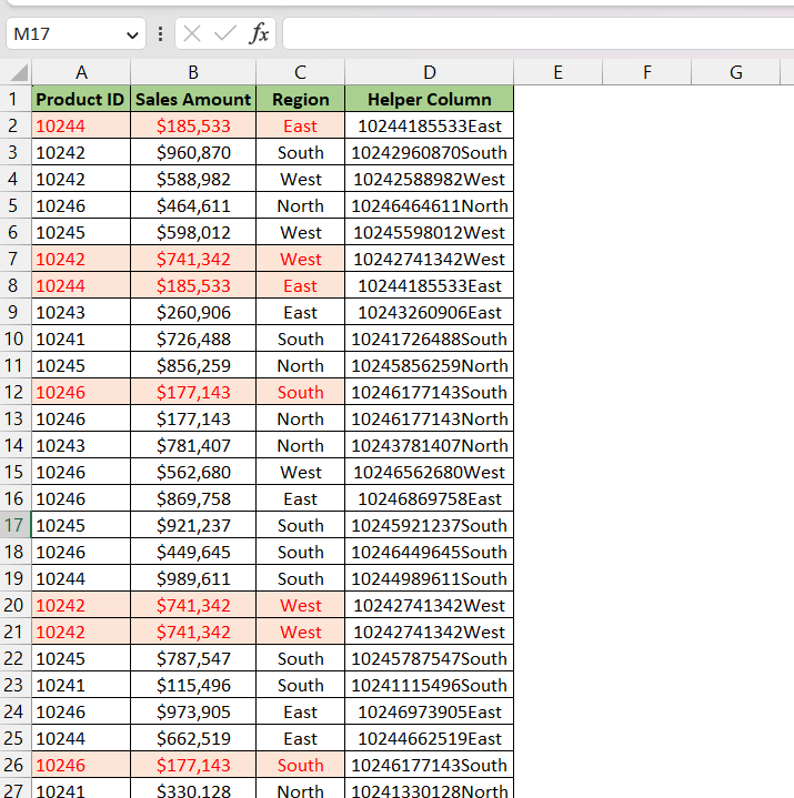
STEP 1: Go to cell D2 and enter the CONCAT function.
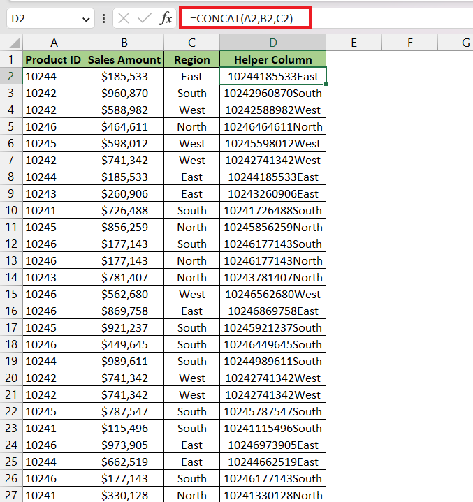
STEP 2: Select all three cells that you want to combine. and copy the formula down.
We will be using range A2:C32 to highlight duplicates and range D2:D32 to check for duplicates.
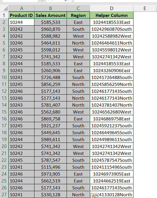
STEP 3: Select the range where you want to highlight duplicates i.e. A2:C32.
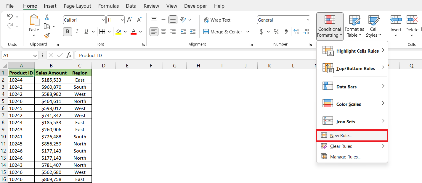
STEP 4: Go to Home > Conditional Formatting > New Rule.
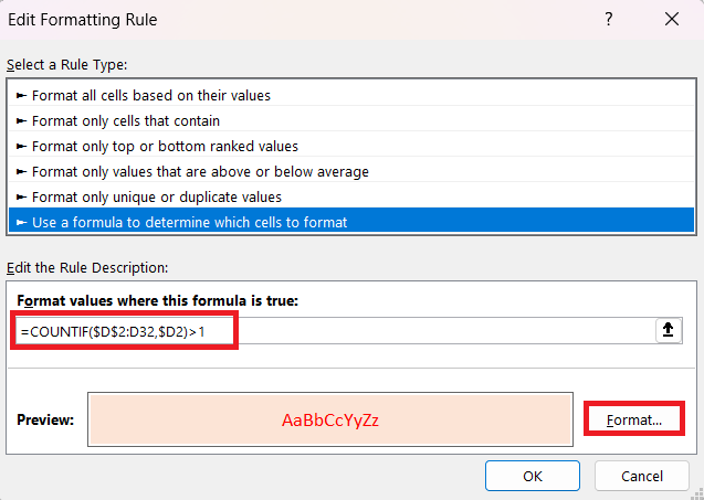
STEP 5: In the New Formatting Rule dialog box, enter the following formula –
=COUNTIF($D$2:D32,$D2)>1
Now, select the formatting that you want and press OK.
All the duplicate rows have been highlighted.
Remove Duplicates
Instead of highlighting duplicates in the list, you may sometimes want to simply remove those duplicates from the list. Let’s see how it can be done:
STEP 1: Select the range containing duplicate values.
STEP 2: Go to Data > Remove Duplicates.
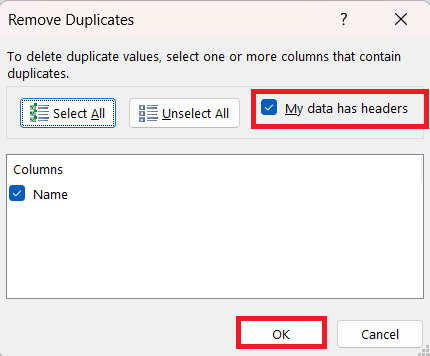
STEP 3: In the dialog box, check My data has headers and click OK.
STEP 4: Excel sends an alert stating the number of duplicates that have been removed and the remaining number of unique values. Click OK.
All the duplicates have been removed and the list now contains only unique values.
Put Unique Values in Another Column
What if we don’t want to highlight duplicates or remove them, we simply want out the unique values in another column?
Excel has a function for this as well- UNIQUE. If you are unable to find this formula, you may be using an older version of Excel. Click here to download Excel 365 and enjoy the benefits of using this amazing function.
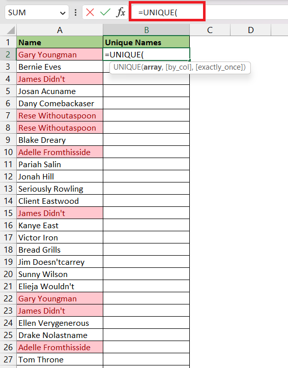
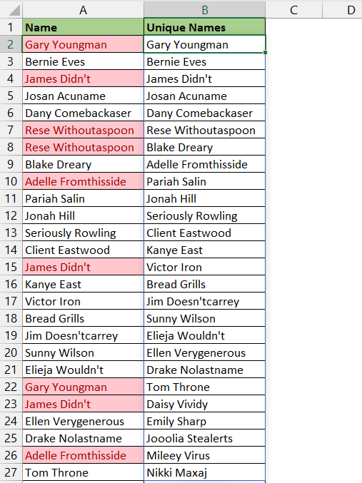
In this example, we have a list of names in column A that contains duplicates. We want to get a list of unique names in column B without making any change in column A. Let’s see how it can be done.
STEP 1: Enter the UNIQUE function in cell B2.
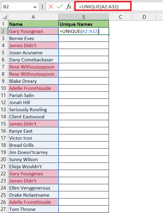
STEP 2: Select the data from which you want to remove duplicates.
All the unique names will be listed in column B.
In this article, we have learned how to highlight duplicate values and rows, how to highlight all except 1st occurrence of duplicates, remove duplicates and get unique values in a new column.
Click here for The BEST Microsoft Excel Tips & Tricks EVER, ranging from Formatting, Macros, Formulas, Tables, Pivot Tables, Working with Data plus Many More!
John Michaloudis is a former accountant and finance analyst at General Electric, a Microsoft MVP since 2020, an Amazon #1 bestselling author of 4 Microsoft Excel books and teacher of Microsoft Excel & Office over at his flagship Academy Online Course.
