In this article, we will cover the following methods to achieve this –
Table of Contents
Let us look at each of these methods in detail.
Download the Excel Workbook below to follow along and understand How to Highlight Every Other Row in Excel –
download excel workbookHighlight-Every-Other-Row.xlsx
Table of Contents
Method 1 – Use CTRL button
If your worksheet does not have many rows, you can hold the CTRL button to highlight the rows that you want. Follow the steps below to learn how to highlight every other row in Excel using the CTRL button –
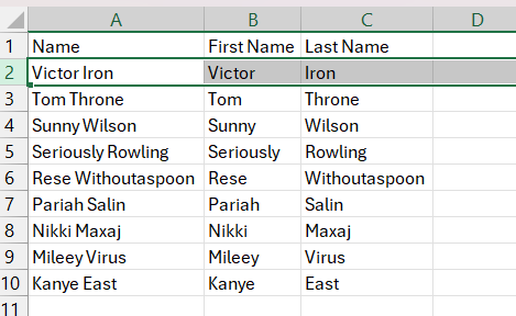
STEP 1: You can select the row number to highlight an entire row.
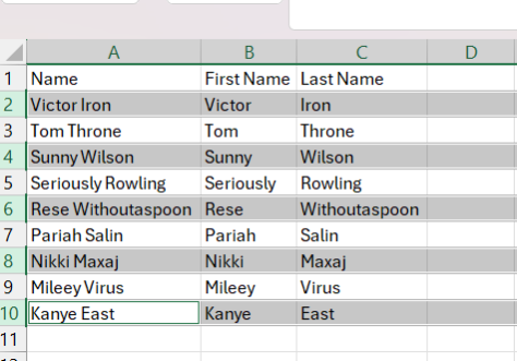
STEP 2: Press CTRL to select additional rows.
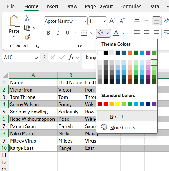
STEP 3: Go to Home > Fill Color > Select an appropriate color.
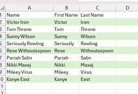
The alternate highlighted rows will be filled with light green color.
Even though this is one of the easiest methods to highlight every other row, using it with a large dataset is not practical.
Method 2 – Format as Table
Another easy way to highlight every other row is to format the data as a table. This will allow you to quickly format a range of cells as a table with a predefined style, including banded rows or columns.
Follow the steps below to highlight alternate rows in Excel by using the Table Format –
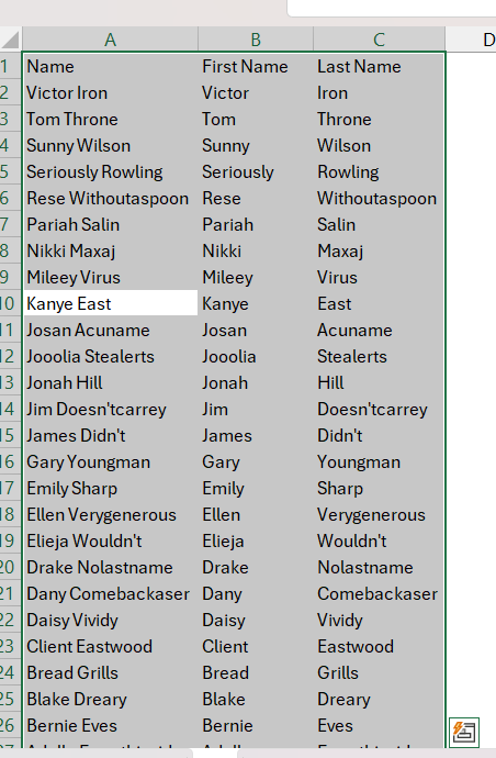
STEP 1: Press CTRL + A to highlight the entire data.
STEP 2: Go to Insert > Table.
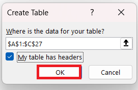
STEP 3: In the Create Table dialog box, check the My table has headers box and click OK.
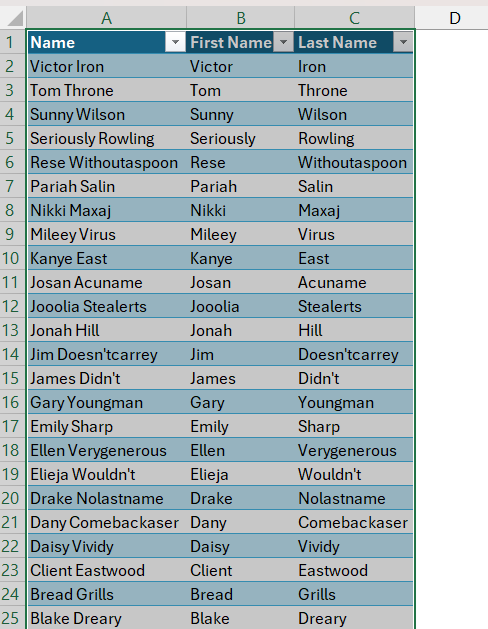
The default blue and white banded rows will be applied to the table range.
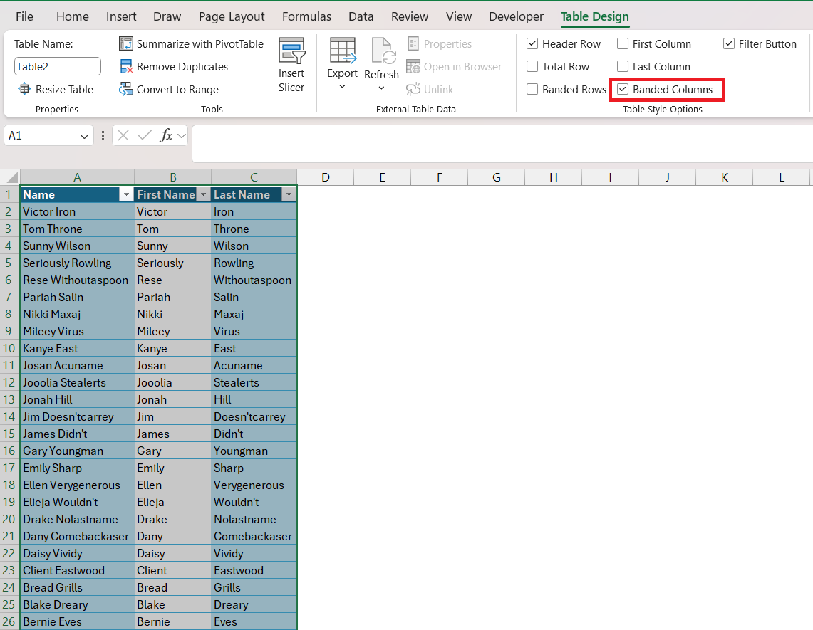
STEP 3: To highlight every other column instead of rows, go to the Tabel Design tab uncheck the Banded Rows option, and check the Banded Columns option.
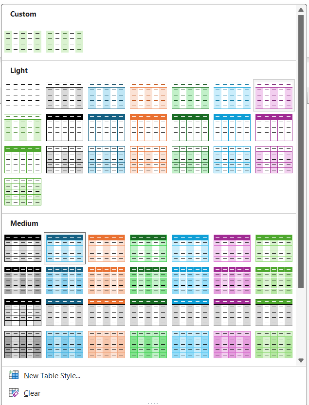
STEP 4: If you don’t like the default color, you can easily change it by clicking on the arrow button next to the Table Style option.
You can select the color option available from the list.
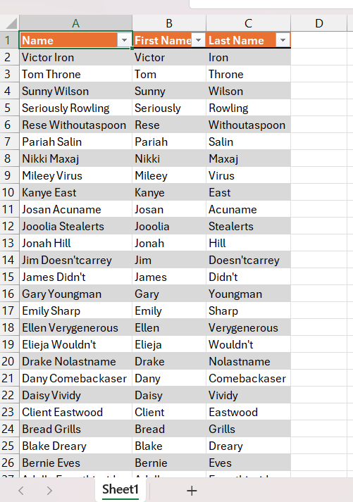
The selected table design will be applied to the data range.
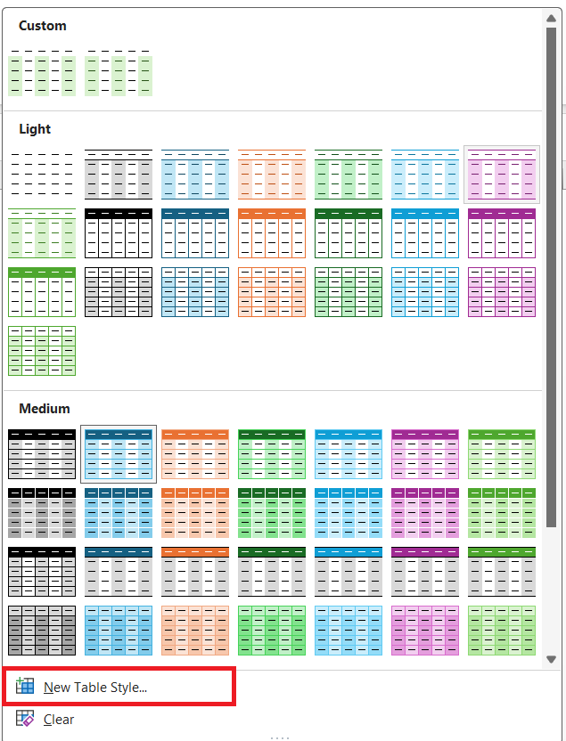
STEP 5: To apply custom formatting, select New Table Style.
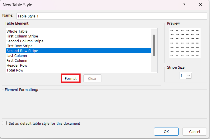
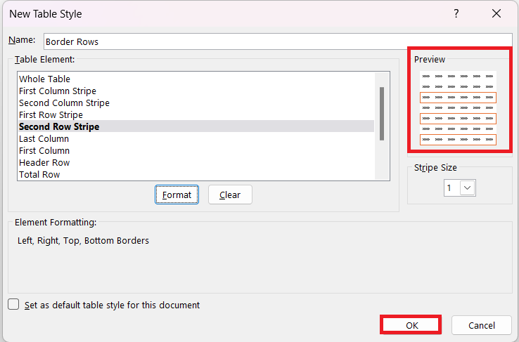
STEP 6: In the New Table Style dialog box, select the Table Element that you want to format and press the Format button.
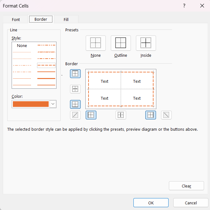
STEP 7: In the Format Cells dialog box, go to Border and select the color and pattern that you want. Press OK.
STEP 8: Double-check the formatting in the Preview section and press OK.
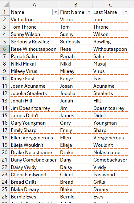
The new formatting will highlight every other row with the selected border.
This is how you can easily highlight rows in Excel.
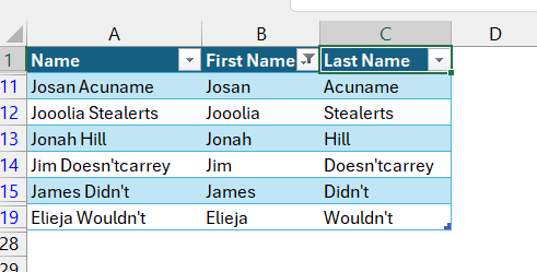
You should know that the formatting that has been applied will adjust automatically even if you sort, remove, or insert new rows. If you filter by the first name starting with “J,” you will notice that the result still displays banded rows.
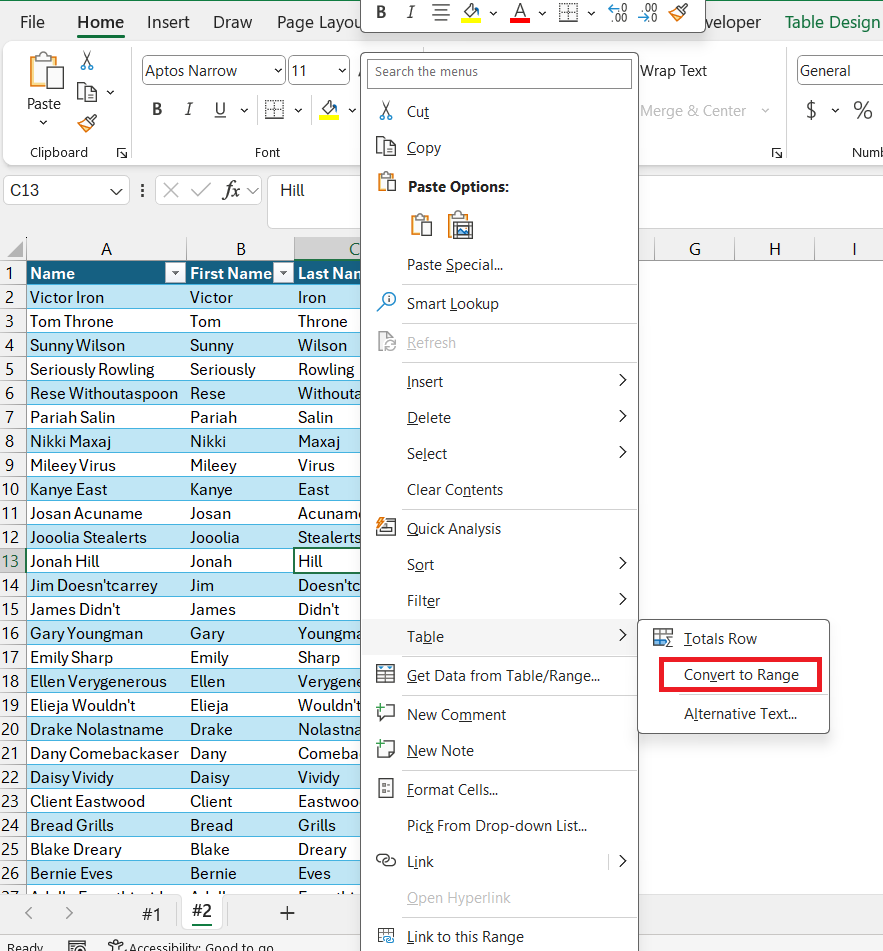
To convert the Table to data range, you can right-click on the table and select Table > Convert to Range.
Even though the table has been converted to range, the formatting remains intact. But, two disadvantages will be faced –
- The formatting will no longer to applied to new rows that you add.
- If you sort or filter data, the formatting will not adjusted and the cells will have the old color only.
Using this method, you can easily highlight alternate rows and columns in Excel. But what if you want to highlight every 3rd or 4th row? This is achievable by following the next method – Conditional Formatting.
Method 3 – Conditional Formatting
Conditional formatting is a feature in Microsoft Excel that allows you to format cells based on specific conditions or criteria. Using this feature, you can highlight every other row or column with colors in Excel.
The formula to be used to highlight every even row using conditional formatting –
=MOD(ROW(),2)=0
where,
- ROW – This function returns the row number of the cell in which the formula is entered.
- MOD – This function calculates the remainder when one number is divided by another. In this case, it calculates the remainder when the row number is divided by 2.
- =0 – This part of the formula checks if the result of the MOD function is equal to zero. If the remainder is zero, it means the row number is divisible evenly by 2, indicating an even row.
This formula is used in conditional formatting to apply a particular format to every other row in a range, creating a banded or striped effect for better visualization of data in tables or lists.
Follow the steps below to highlight every other row in Excel –
STEP 1: Press CTRL + A to highlight the entire data.
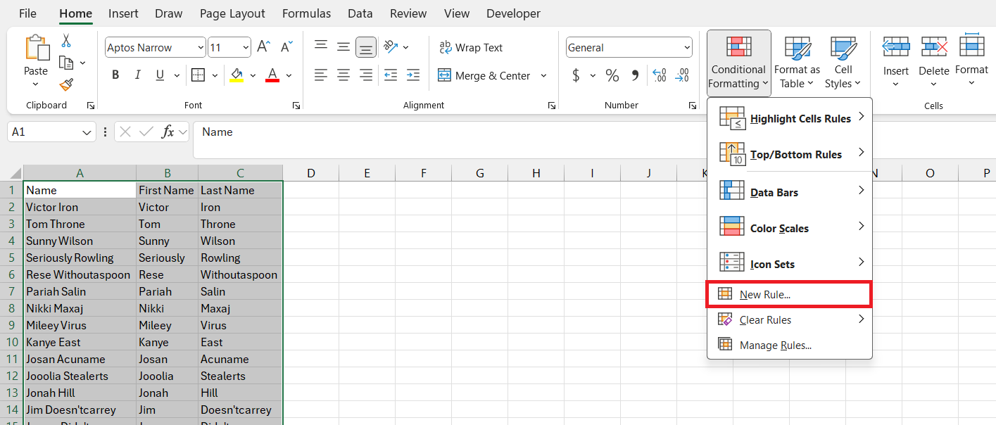
STEP 2: Go to Home > Conditional Formatting.
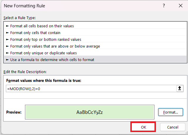
STEP 3: From the submenu, choose New Rule to open the New Formatting Rule dialog box.
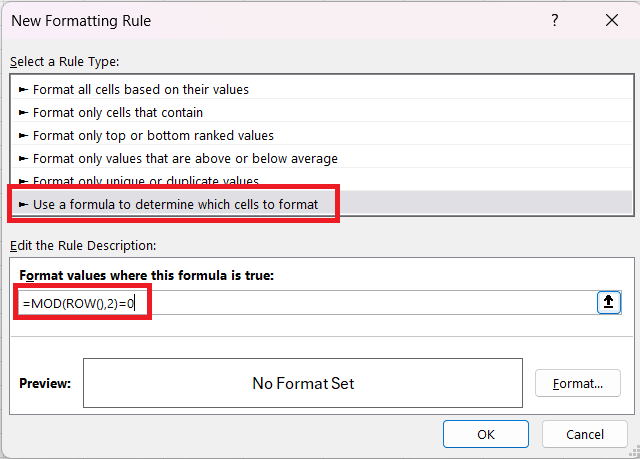
STEP 4: In the New Formatting Rule dialog box,
- Select Use a formula to determine which cells to format.
- Type the formula – MOD(ROW(),2)=0
- Select Format.
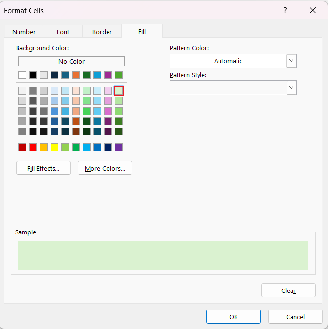
STEP 5: Under the Fill section, select the light green color and press OK.
STEP 5: Double-check the format in the Sample section and press OK.
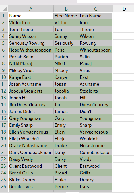
The selected formatting will be applied to the table range.
- To highlight odd rows, you can use the formula: MOD(ROW(),2)=1
- To highlight alternate columns, you can use the formula: MOD(COLUMN(),2)=0
- To highlight every nth row in Excel, use the formula: MOD(ROW(),n)=0.
Conclusion
Microsoft Excel provides various methods to enhance data presentation, and one common formatting technique is to highlight every other row for improved readability. The article covered three methods for achieving this – holding the CTRL button to manually highlight rows, formatting data as a table for banded rows or columns, and using conditional formatting to highlight every nth row or column.
Learn our Top 7 Excel Interview Questions to Land Your Dream Job!
John Michaloudis is a former accountant and finance analyst at General Electric, a Microsoft MVP since 2020, an Amazon #1 bestselling author of 4 Microsoft Excel books and teacher of Microsoft Excel & Office over at his flagship Academy Online Course.
