Microsoft Excel Design Hacks reveals the transformative power of how to add borders in spreadsheets. Borders do more than delineate; they guide users, emphasize key data, and enhance aesthetics, making complex tables navigable and visually appealing. Learning to apply and customize borders can elevate the presentation and functionality of your Excel worksheets.
Key Takeaways:
- Borders in Excel serve a dual purpose: improving readability and adding visual appeal to spreadsheets.
- Adding standard borders is straightforward and can significantly enhance the appearance of your cells with just a few clicks.
- Custom border styles allow for personalized spreadsheet designs, offering creative control over aesthetics.
- Adjustments to border color and width are essential for highlighting critical information or sections within your data.
- Efficient use of keyboard shortcuts and strategic application of border styles can streamline your workflow and make your data presentation more effective.
Table of Contents
Introduction to Excel Design Hacks
The Importance of Borders in Excel
They can guide users through complex data tables, highlight critical information, and make your worksheets look polished and professional. Think of cell borders as the unsung heroes of spreadsheet navigation, often overlooked but vital in crafting an easily digestible document.
Enhancing Readability and Aesthetics
Borders serve not only a practical purpose but also add an element of design to your spreadsheets. A well-placed border can break up large chunks of data, making them easier to read and follow. When you use borders thoughtfully, they accentuate the aesthetics of your document, ensuring that your data is not just understood but also pleasing to the eye.
Mastering Basic Border Applications
Adding Standard Borders to Excel Cells
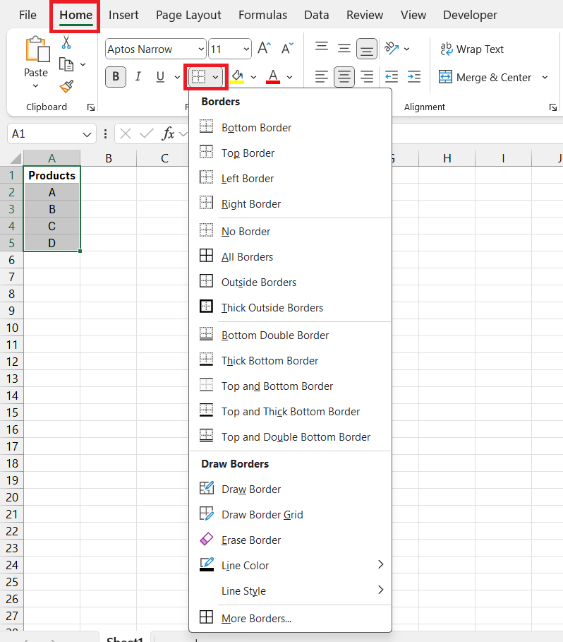
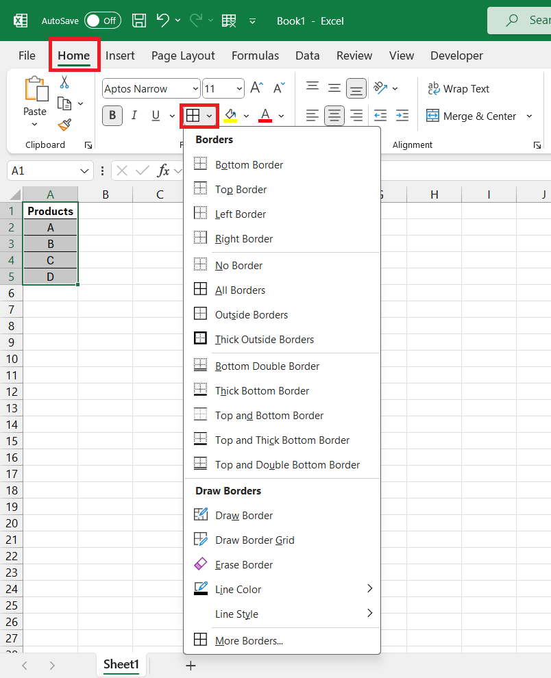
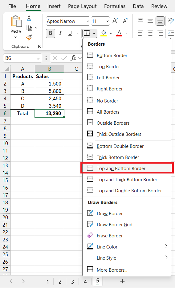
To kick things off with standard borders, it’s really quite simple. Once you’ve highlighted the cells where you want to spruce things up, head over to the “Home” tab, and look for that “Borders” option nestled in the Font group. Here’s a quick step-by-step guide:
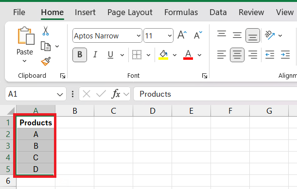
STEP 1: Select the cells you want to frame.
STEP 2: Click “Borders” in the “Home” tab under the Font group.
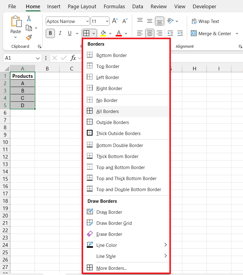
STEP 3: Choose from several predefined borders like “All Borders,” “Outside Borders,” or “Bottom Border.”
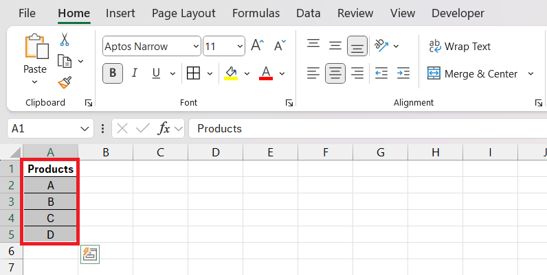
This feature offers an instant makeover to your cells, so they stand out without any fuss.
Removing Borders with Ease
Just as they’re swiftly applied, removing borders in Excel is a breeze. When you need a clean slate, simply:
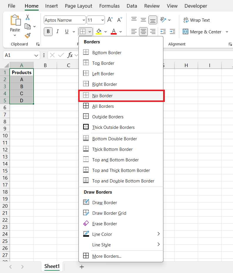
STEP 1: Highlight the cells whose borders you wish to bid farewell.
STEP 2: Click on the “Home” tab and find your way to the “Borders” dropdown again.
STEP 3: Select “No Border” and watch the lines vanish, leaving a borderless canvas.
Following these steps declutters your spreadsheet, ensuring the focus is only where you want it.
Advanced Border Customizations
Creating Your Own Border Styles
Unleashing your creative side in Excel is easy with custom border styles. Follow these steps if you’re ready to design a border that’s uniquely yours:
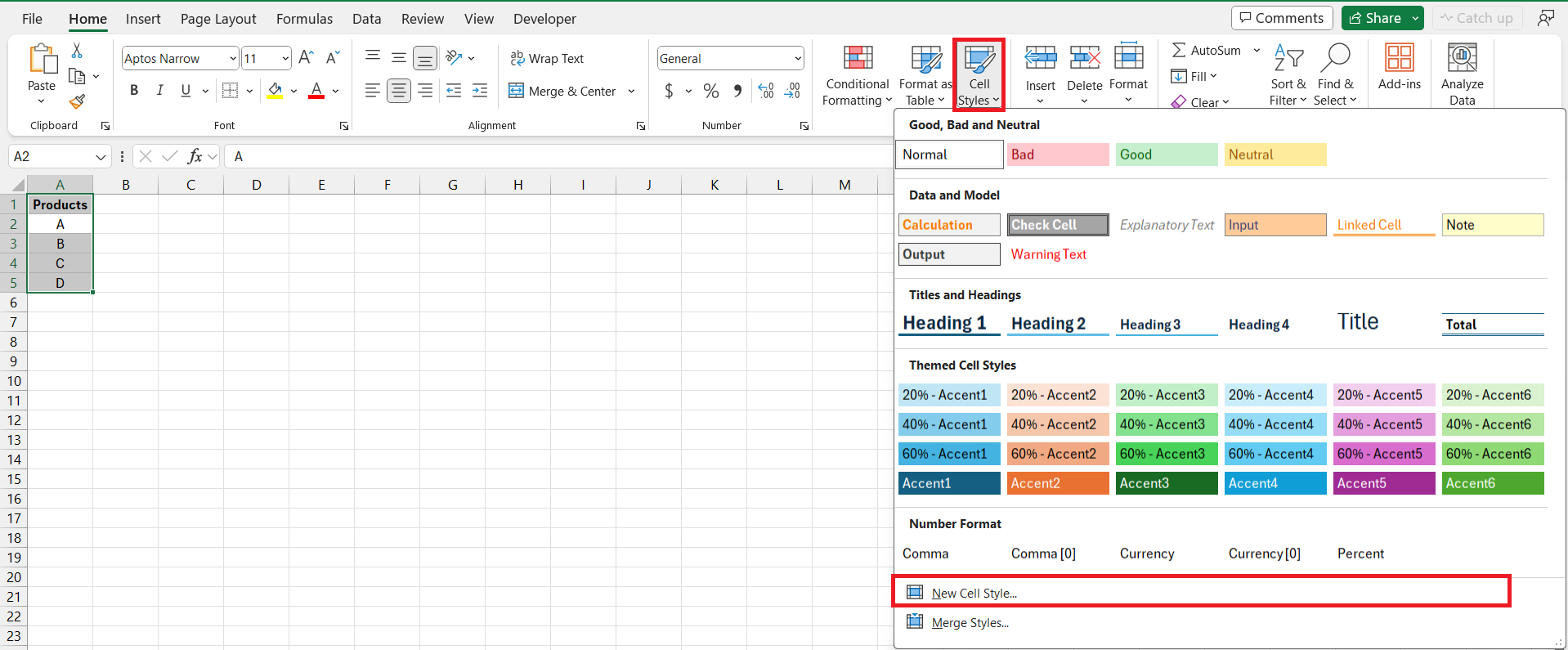
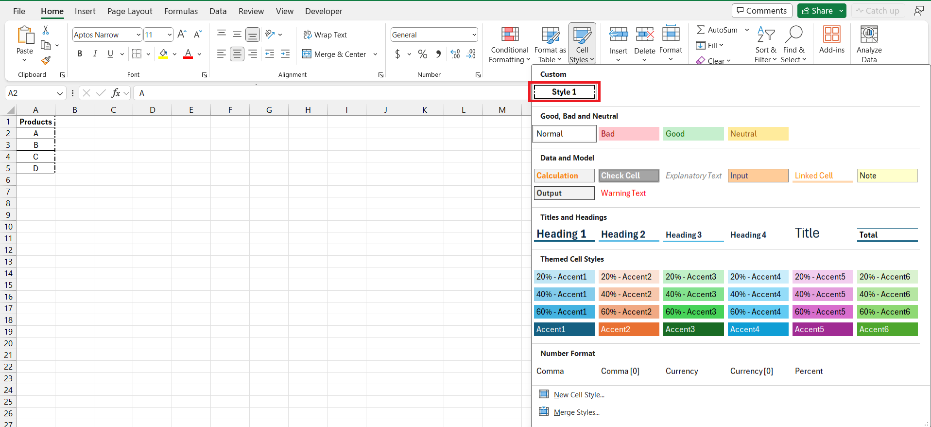
STEP 1: Choose “Cell Styles” from the “Styles” group on the “Home” tab. Then select “New Cell Style”.
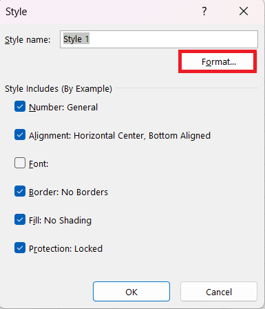
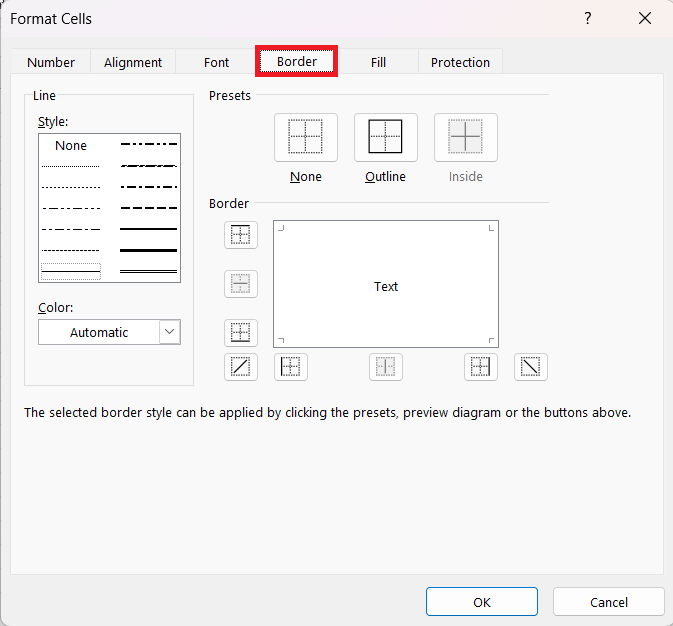
STEP 2: Give this new style a name that resonates with its purpose and hit “Format” button.
STEP 3: Swing on over to the “Border” tab.
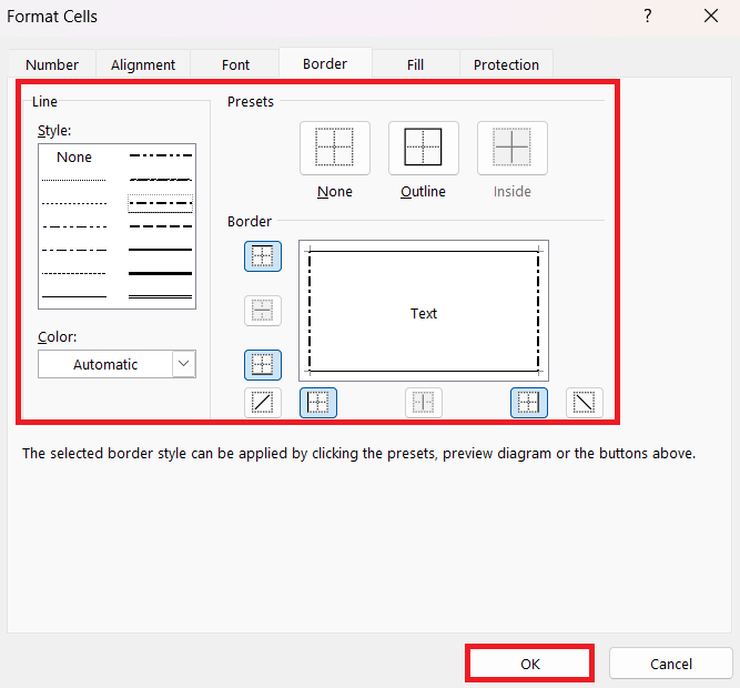
STEP 4: Mix and match line styles and colors, then apply them to your chosen border edges.
STEP 5: Press “OK” and enjoy your handiwork. Choose your custom style in case if needed.
Creating a custom style lets you apply your signature border consistently across multiple spreadsheets.
Color and Width Adjustments for Emphasis
When the standard black and white borders just won’t cut it, adding a splash of color and altering the width can be just the ticket. These adjustments help emphasize particular data or sections of your spreadsheet:
STEP 1: Highlight the cells.
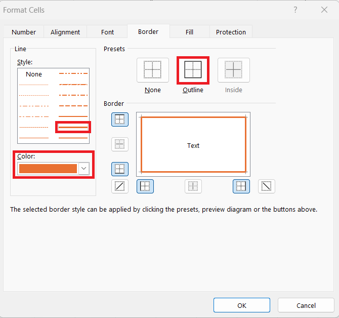
STEP 2: Right-click and pick “Format Cells” or press Ctrl + 1. And navigate to the “Border” tab in the dialog box.
STEP 3: Select your desired line style and then pick the color that strikes your fancy. Opt for a thicker line for more substantial emphasis or a subtle thin line for a gentle nudge of attention.
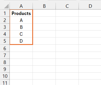
An orange colored outline border will be added to the selected cells.
Remember, color and width are potent tools; use them sparingly to draw the eye without creating visual clutter.
Efficiency Tips for Border Formatting
Keyboard Shortcuts for Speedy Border Application
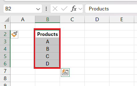
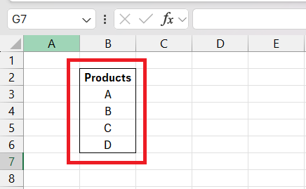
Getting familiar with keyboard shortcuts can make border applications a speedy affair. For example, adding an outline border around the selected cells is efficient when you:
STEP 1: Select your cells.
STEP 2: For Windows, press Ctrl + Shift + &. For Mac, use Command + Option + 0.
These shortcuts add an instant border using the default line style and thickness, dramatically speeding up your workflow.
Visual Tricks with Borders
Delineating Data Using Top and Thick Bottom Borders
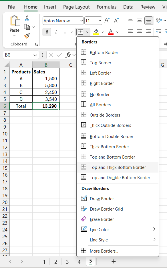
When your spreadsheet data needs clear defining lines, using top and thick bottom borders adds that well-defined separation. It’s an effective way to delineate title rows from data or to mark off summarized sections:
STEP 1: Highlight the row or cell where you want the delineation and navigate to the “Borders” dropdown in the “Home” tab.
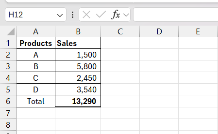
STEP 2: Select “Top and Thick Bottom Border” for that distinct visual demarcation.
STEP 3: Check the result.
This gives your headers prominence and neatly sections off parts of your dataset, compelling the reader’s eye to follow the intended flow of information.
Applying Gridlines for Clarity
To aid in data readability and maintain a clean workspace, applying gridlines in Excel is key. Here’s a quick guide:
STEP 1: Navigate to the “View” tab at the top of your Excel worksheet.
STEP 2: Locate the “Show” options and check the “Gridlines” box to make them visible on screen.
STEP 3: If you need to print the spreadsheet with gridlines, switch over to “Page Layout”, find “Sheet Options”, and under “Gridlines”, select “Print”.
This simple action can transform a block of data into a neatly organized grid, making it significantly easier to navigate rows and columns at a glance.
Frequently Asked Questions
How do I add a border to every other row in Excel?
To add a border to every other row in Excel, use the ‘Format as Table‘ feature or conditional formatting. First, select your data range, then go to the ‘Home’ tab, and choose ‘Format as Table’ for predesigned styles. For a more customized approach, use conditional formatting with a formula to apply borders to alternate rows.
How do I apply a custom border style in Excel?
To apply a custom border style in Excel: select cells, click “Home”, “Cell Styles”, “New Cell Style”. Name it, hit “Format”, pick line styles and colors on “Border” tab, apply, click “OK”. Your new style is now under “Cell Styles” for future use.
Can I add borders to multiple cells at once?
Yes, you can add borders to multiple cells at once in Excel. Simply select the range of cells where you want the borders, then apply your chosen border style to the whole selection using the Borders option in the Home tab.
How do I change the color and width of cell borders?
To change the color and width of cell borders in Excel, select your cells, press Ctrl + 1 for “Format Cells”, go to “Border” tab, pick a color and line style. Adjust width by selecting a thicker style. Click “OK” to apply.
What’s the quickest way to remove all borders in an Excel worksheet?
The quickest way to remove all borders in an Excel worksheet is to select the cells or range, go to the “Home” tab, click on “Borders” in the “Font” group, and choose “No Border”. This will clear all borders instantly.
John Michaloudis is a former accountant and finance analyst at General Electric, a Microsoft MVP since 2020, an Amazon #1 bestselling author of 4 Microsoft Excel books and teacher of Microsoft Excel & Office over at his flagship Academy Online Course.
