How to Insert Checkbox in Excel in 5 Easy Steps

A Checkbox in Excel is a form control that can be used to select or deselect an option by simply clicking on it. When you select a checkbox, a small x mark appears indicating that the option has been selected. If the box is empty, the option is not selected.

It can be used for creating checklists, form inputs, interactive charts, reports, dashboards, and much more.

In this article, you will be covering the following Checkbox in Excel topics in detail –

• Activate Developer Tab
• Insert a Checkbox in Excel
• Insert Multiple Checkboxes in Excel
• Link Checkbox to a Cell
• Examples of Using Checkbox in Excel
• Delete Checkbox in Excel

Let’s look at each of these topics one by one!

Make sure to download this Excel Workbook and follow along:

download excel workbookExcel-Checkbox.xlsx

 

Activate a Developer Tab

The only way to create a checkbox is by using the Developer tab option. If it is not visible on your ribbon, follow the steps below to add it –

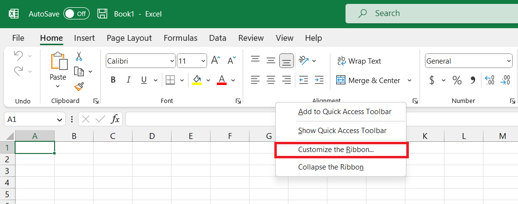
STEP 1: Right-click anywhere on your Ribbon and select Customize the Ribbon.

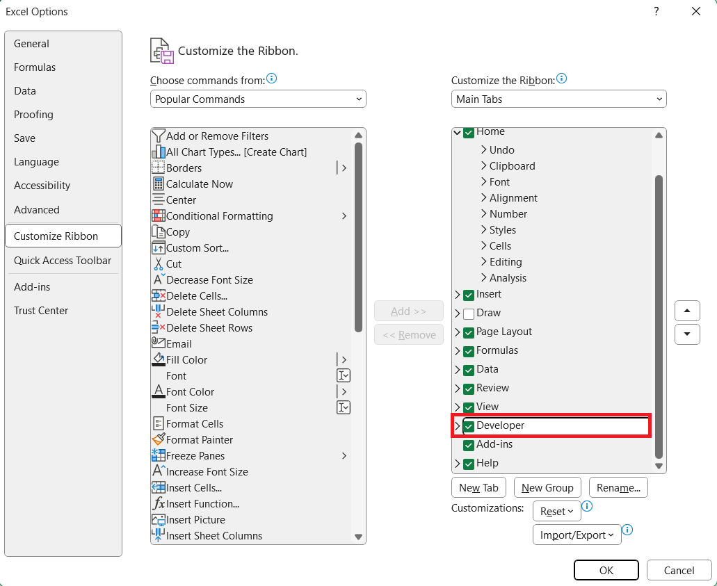
STEP 2: Make sure the Customize Ribbon is selected. Then select the Developer option under Main Tabs.

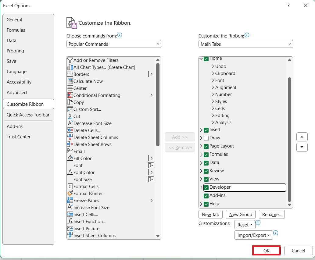
STEP 3: Click OK.

The Developer tab will now show up on the ribbon.

 

Insert a Checkbox in Excel

Once you have the Developer tab visible on your ribbon, you can follow the steps below to insert a Checkbox in Excel –

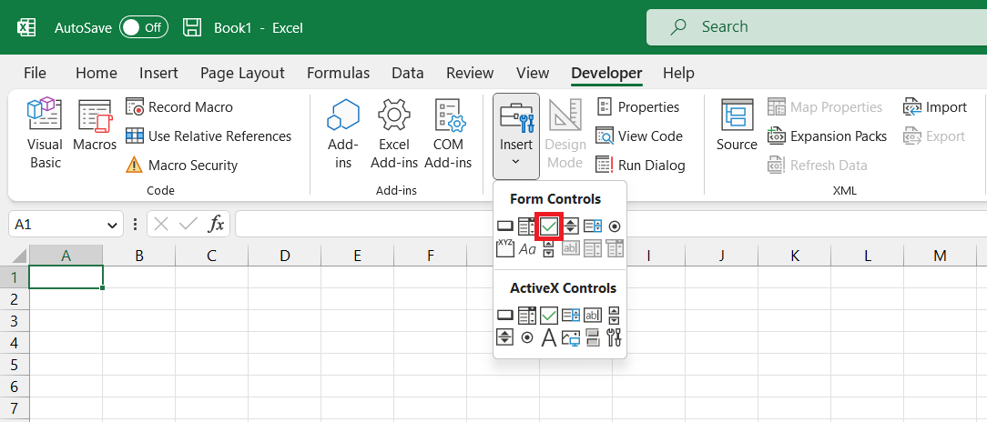
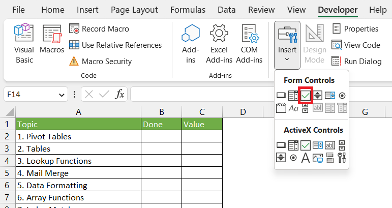
STEP 1: Click on Developer Tab.

STEP 2: Under the Controls, Click on Insert.

STEP 3: Click on the Checkbox icon under Form Controls (small box with a blue tick).

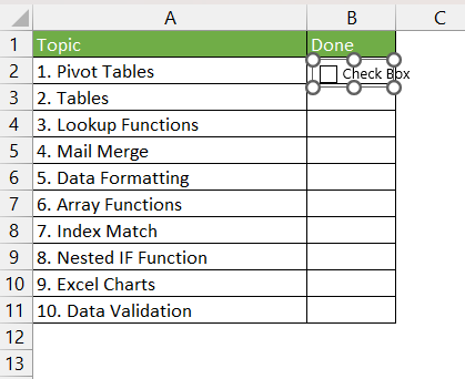
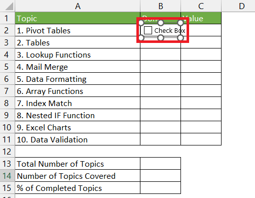
STEP 4: Click anywhere on the sheet, and the checkbox will be inserted there.

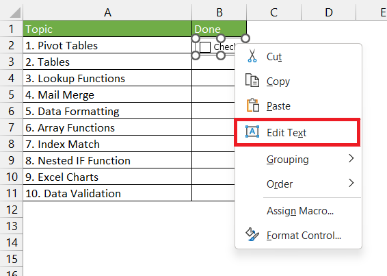
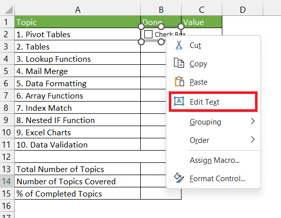
STEP 5: Right-click and select Edit Text. You can edit or remove text as needed.

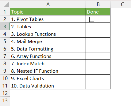
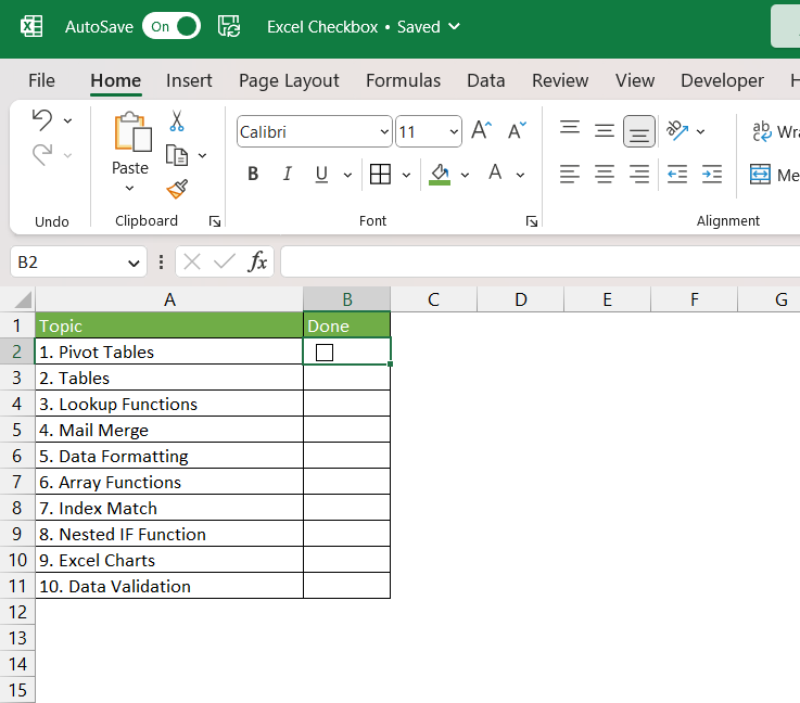
The checkbox is now ready!

 

Insert Multiple Checkboxes in Excel

Now that you have added a checkbox to cell B2 – How do you insert them for the remaining cells?

If you try to add the checkboxes one by one using the method shown above it will be a time-consuming process. There are 2 ways in which you can quickly add multiple checkboxes to your Excel worksheet.

Let’s look at them.

Method 1 – Copy Paste

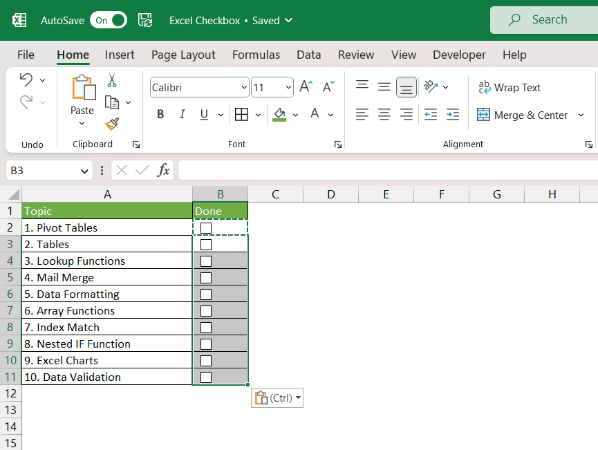
You can simply copy the checkbox added in cell B2 and paste them into the required range.

• Select the cell containing the checkbox
  
• Press Ctrl  + C to copy it.
  
• Select the cells where you want to paste and then press Ctrl + V.
  

You can also highlight all the cells and use the keyboard shortcut Ctrl + D to achieve the same result!

 

Method 2 – Drag and Fill

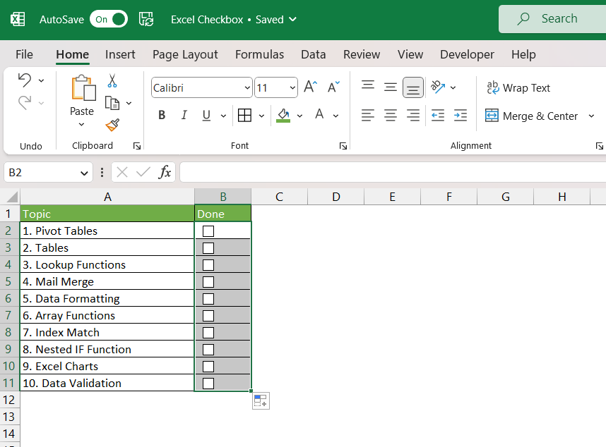
In this method, you can select the cell containing the checkbox and then move your cursor to the bottom right corner of the cell. The arrow will convert into a thin black cross icon.

Now, simply drag and fill the checkboxes to the cells below.

 

 Link Checkbox to a Cell

You can link the value of the checkbox to a cell address in your worksheet. When you select the checkbox, the value in the linked cell will display TRUE otherwise it will display FALSE.

You can use this value in the cell to perform various actions like conditional formatting, creating interactive charts or reports, hiding or unhiding rows/columns, etc. Let’s see how you can link a checkbox to a cell:

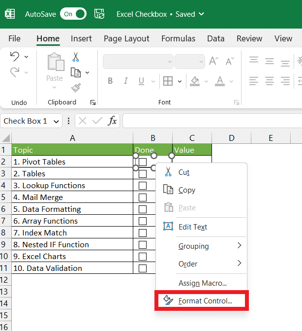
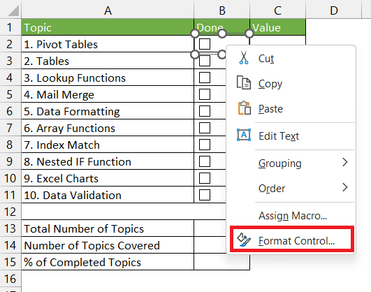
STEP 1: Right-click on the checkbox and select Format Control.

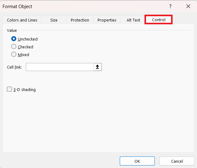
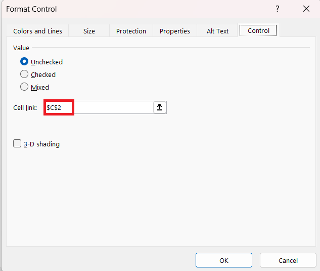
STEP 2: In the Format Object window, go to Control Tab.

STEP 3: Under the Cell link, select the cell where you want the value to be displayed. Here, it is cell C2.

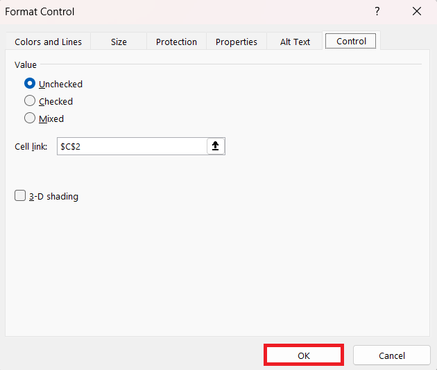
STEP 4: Click OK.

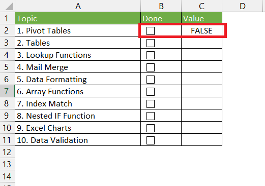
You can see that since the checkbox is not selected, the value in cell C2 is showing FALSE.

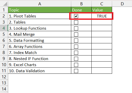
Once you select the checkbox, the value will change to TRUE.

 

Example of Using Checkbox in Excel

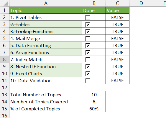
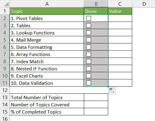
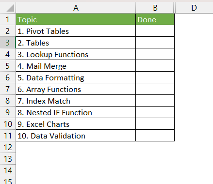
In this example, you have a list of topics that needs to be covered by a student. You need to use the checkboxes in Excel to track the progress and provide a summary for the same.

You also have to strikethrough the topics that have been completed and add a green color fill to them. This can be achieved using the Conditional Formatting option in Excel.

STEP 1: Go to Developer Tab > Insert > Checkbox.

STEP 2: Click on cell B2 to insert the checkbox in that cell.

STEP 3: Right-click and select Edit Text. Clear the text.

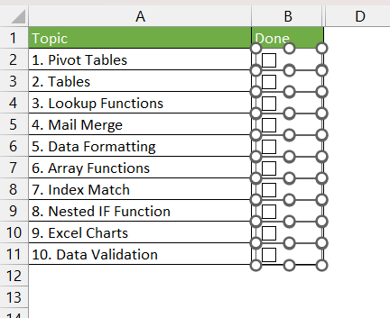
STEP 4: Drag and fill the checkboxes in range B3:B11.

STEP 5: Right-click on the checkbox and select Format Control.

STEP 6: Select cell C2 in the cell link option.

STEP 7: Do this for all the checkboxes.

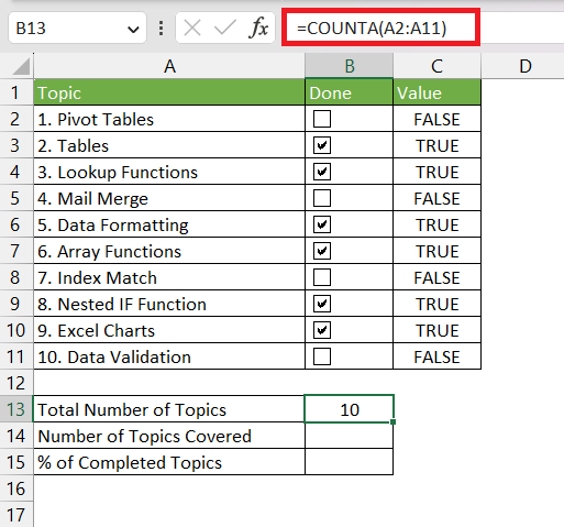
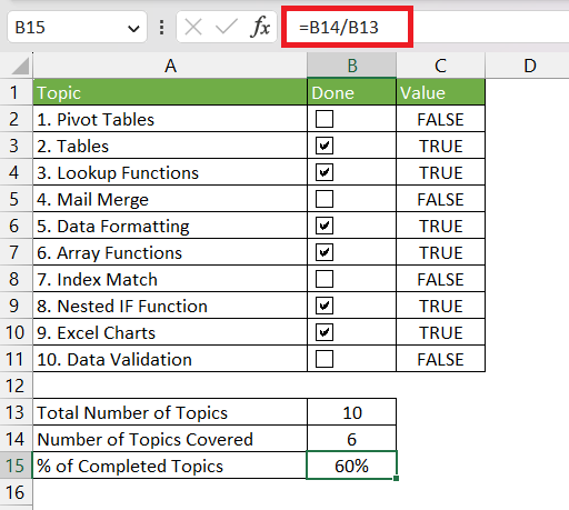
STEP 8: In cell B13, insert the COUNTA formula to get the total number of topics covered.

=COUNTA(A2:A11)

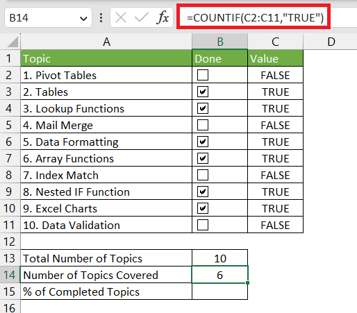
STEP 9: In cell B14, insert the COUNTIF function to get the total number of TRUE in range C2:C11. These cells will display TRUE only when the checkbox is selected indicating that the topic has been covered.

=COUNTIF(C2:C11,”TRUE”)

STEP 10: In cell B15, to get the percentage of topics covered simply divide B14 by B13.

=B14/B13

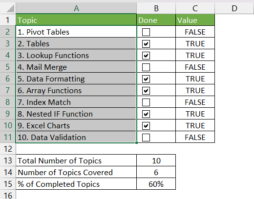
STEP 11: To add conditional formatting, select the cell range where you want the formatting to be shown. Here, it is cell A2:A11.

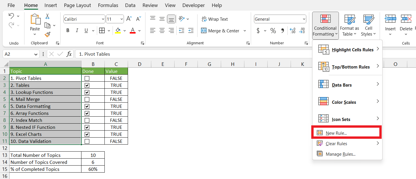
STEP 12: Go to Home > Condition Formatting > New Rule.

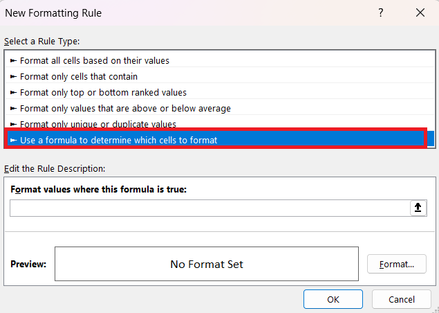
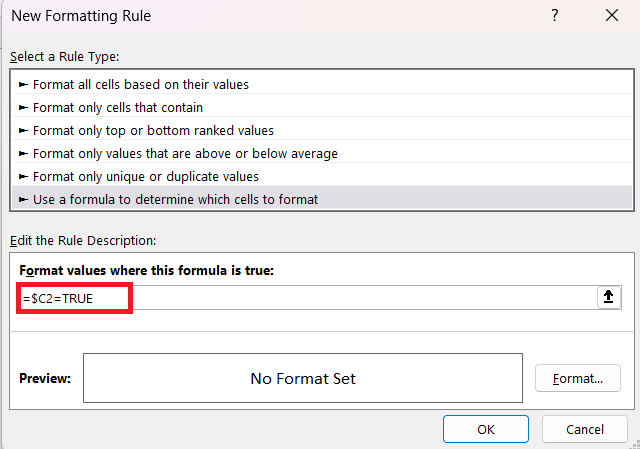
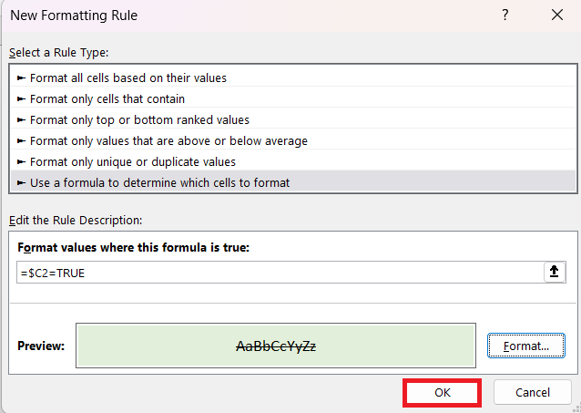
STEP 13: In the New Formatting Rule dialog box, select Use a formula to determine which cells to format.

STEP 14: Type the formula stated below –

=$C2=TRUE

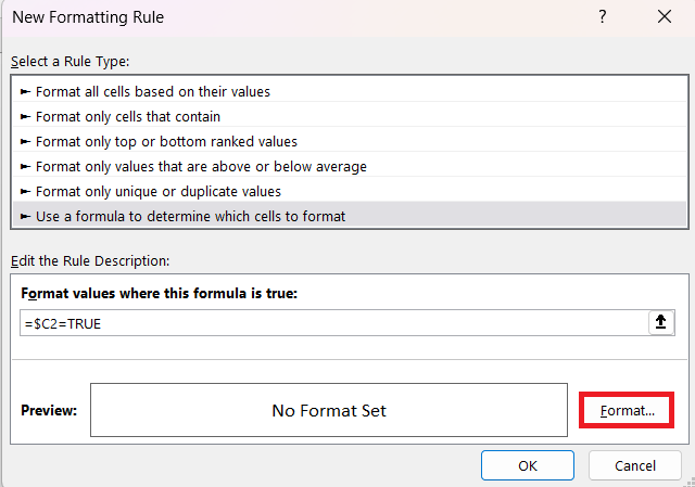
STEP 15: Click on the Format button.

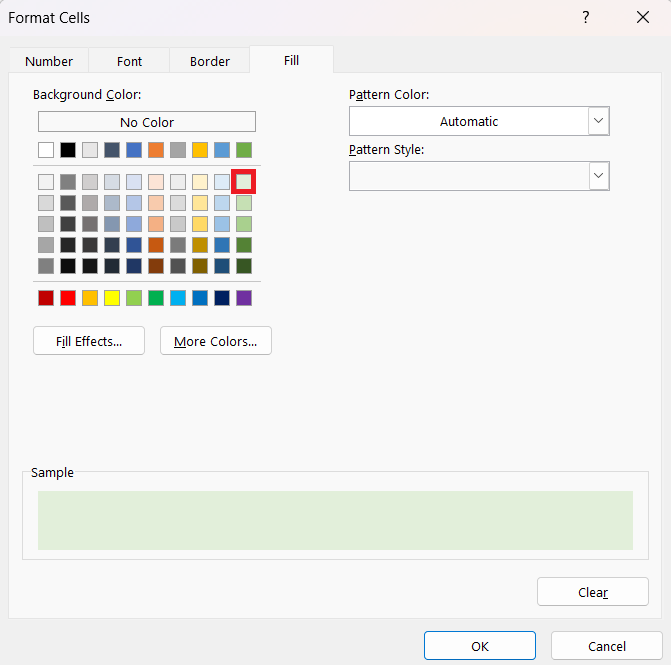
STEP 16: Under the Fill tab, select the light green color.

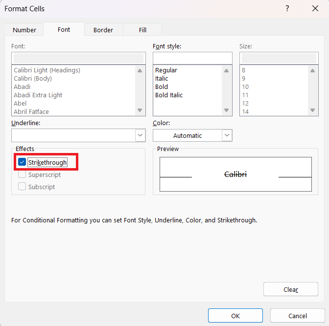
STEP 17: Under the Font tab, select Strikethrough.

STEP 18: Double-check the result under Preview and then click OK.

And Voila, you will see that the desired result has been achieved. The topics that have been marked as completed in the checkbox are strikethrough and highlighted in green as well.

 

Delete Checkbox in Excel

Deleting a single checkbox is a straightforward task but deleting multiple checkboxes in your worksheet can become tedious. You can follow any of the following methods below to delete multiple checkboxes at once:

Method 1: Use the Ctrl key

• Press and hold the Ctrl key on your keyboard and select all checkboxes.
  
• Press the Delete button on your keyboard.

All the selected checkboxes will be deleted.

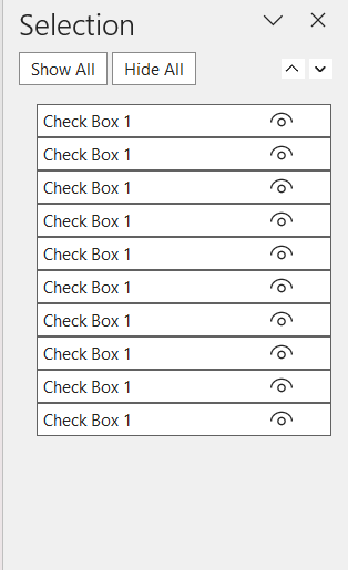
Method 2: Use the Selection Pane

• Go to Home > Find & Select.
  
• In the dropdown, click on Selection Pane.
  
• In the Selection Pane, select the checkboxes you want to delete.
  
• Press the Delete button on your keyboard.

All the selected checkboxes will be deleted.

 

Method 3: Use the Go To Special option

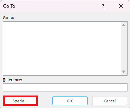
• Press Ctrl + G to open the Go To dialog box. Select Special.
  
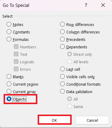
• In the Go to Special dialog box, select Objects. Click OK.
  
• All the checkboxes will be selected.
  
• Press Delete.

All the selected checkboxes will be deleted.

The only limitation of this method is that all objects in the active worksheet including shapes, charts, dropdowns, etc. will be deleted.

 

Conclusion

A Checkbox is a very useful feature in Excel that allows users to select or deselect an option. It is helpful as it prevents users from manually entering data hence reducing the scope of error. It can be used for creating forms, checklists, interactive charts, reports, etc.

In this article, we have covered how to insert single or multiple checkboxes in Excel, link the value to a cell, and delete them as well.

For more tips and tricks to master Excel, check our Excel online classes below!