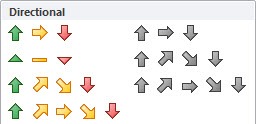
An Icon Set is a Conditional Formatting icon/graphic that you can include in your cells or Pivot Tables.
The icon will depend on the cell´s value so you can highlight key variances or trends. There are a few sets that you can include, like:
DIRECTIONAL (Change in values)
SHAPES (Milestones)
INDICATORS (Positive/Negative)
RATINGS (Scores)
I show you how easy it is to insert an Icon Set within a Pivot Table that will show a “directional icon” depending on the change of the monthly sales values.
So when monthly sales increase from the previous month, a green up arrow is shown and when monthly sales decrease, a red down arrow is shown.
STEP 1: Place the SALES Field in VALUES
STEP 2: Click on the new field and Select Value Field Settings
Go to Show Values as > Difference From > (previous) to get the difference from the previous month
STEP 3: Click in a variance cell. Go to Home > Styles > Conditional Formatting > Icon Sets > The First Icon Set
STEP 4: Make sure to select the third option. This excludes the subtotals and grand totals.
STEP 5: Go to Home > Styles > Conditional Formatting > Manage Rules
Select Edit Rule.
Set the settings to the ones shown below. This will set the column to show the arrow icons only.
Your icons are now ready in your Pivot Table!
How to Use Icon Sets In A Pivot Table
HELPFUL RESOURCE:
John Michaloudis is a former accountant and finance analyst at General Electric, a Microsoft MVP since 2020, an Amazon #1 bestselling author of 4 Microsoft Excel books and teacher of Microsoft Excel & Office over at his flagship Academy Online Course.


