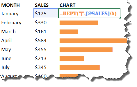
When you are creating an Excel Dashboard and are limited by space and do not want to insert a chart, you can easily create an in-cell bar chart using the REPT (repeat) function.
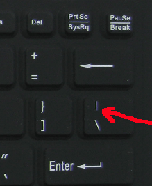
The REPT function uses the vertical bar character | as the first argument: text and references the value cell for the second argument: number_times
So it enters the vertical bar character by the amount of times of the value cell, looking something like this:
||||||||||||||||||||||||||||||||||||||||||||||||||||||||||||||||||||||||||||||||||||||||||||||
Here is how it is done in just a few steps:
Download excel workbookREPT-Function-Column-Chart.xlsx
STEP 1: Enter the REPT function in a column next to your values
=REPT(text,number_times)
STEP 2: Enter the vertical bar keyboard character in the first argument =REPT(“|”)
STEP 3: Reference the value cell for the second argument =REPT(“|”, a1)
STEP 4: Highlight the formula column and insert the Stencil font from the Home menu and choose a font color
STEP 5: If your value cells are high, the bar will go out of your screen. To fix this, you need to enter a divisor in the second argument of your formula which will reduce the length eg =REPT(“|”,a1/5)
John Michaloudis is a former accountant and finance analyst at General Electric, a Microsoft MVP since 2020, an Amazon #1 bestselling author of 4 Microsoft Excel books and teacher of Microsoft Excel & Office over at his flagship Academy Online Course.


