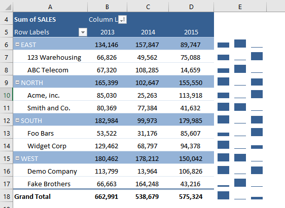
Once you have your Pivot Table ready and setup, you want to add something more graphical beside your data points. We have just the thing for you, you can include sparkline with pivot tables!
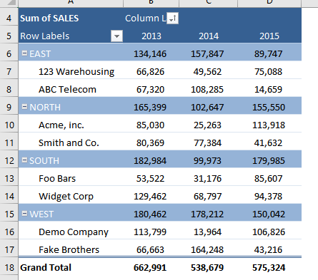
Here we have our Pivot Table ready:
See how you can do this in just a couple of steps.
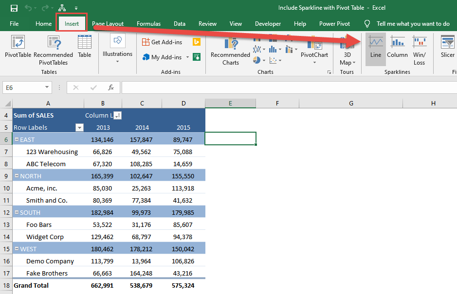
STEP 1: Select a spot right beside your Pivot Table. Go to Insert > Sparklines > Line
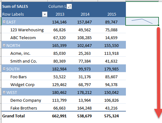
We want to create a sparkline based on our first row of data. Select the sales values of 2013-2015. Then click OK.
STEP 2: On the lower right corner, drag it all the way down to populate the rest of your table with sparklines.
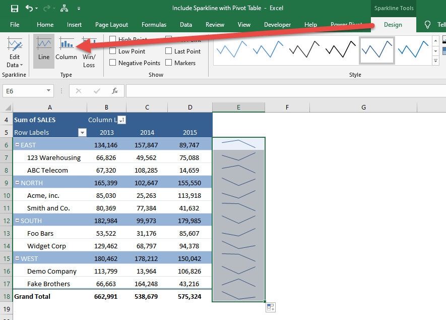
STEP 3: We can change the type as well. Go to Sparklines Tools > Design >Type > Column
You now have sparklines for your Pivot Table!
How to Include Sparkline with Pivot Table
Helpful Resource:
Bryan
Bryan is a best-selling book author of the 101 Excel Series paperback books.
