INDEX and MATCH are the go-to Excel functions for carrying out sophisticated lookups, owing to their high degree of flexibility. With these functions, you can execute both vertical and horizontal lookups, 2-way lookups, left lookups, case-sensitive lookups, and even perform lookups based on multiple criteria. To enhance your Excel abilities, it is recommended that you add INDEX and MATCH to your skill set. Below are numerous examples to help you get started.
This article offers a straightforward guide on utilizing INDEX and MATCH together to execute lookups. It adopts a methodical approach by first outlining the individual functions of INDEX and MATCH, and then demonstrating how to merge both functions to achieve a versatile two-way lookup. You will also find more advanced examples later on in the article.
Here are some of the techniques we will explore:
- The INDEX Function
- The MATCH Function
- INDEX and MATCH together
- Two-way lookup with INDEX and MATCH
- Left Lookup
- Case-sensitive Lookup
Let’s look at each of these ways thoroughly!
The INDEX Function
Excel’s INDEX function is a remarkably flexible and potent tool that is featured in many advanced formulas. So, what does INDEX do? Simply put, it retrieves the value at a specific position in a range.
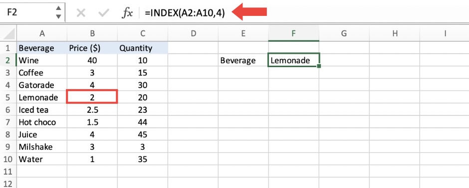
To illustrate, suppose you have a list of beverages in your menu, and you wish to obtain the name of the beverage, which is Lemonade, using a formula. You can utilize INDEX in the following way
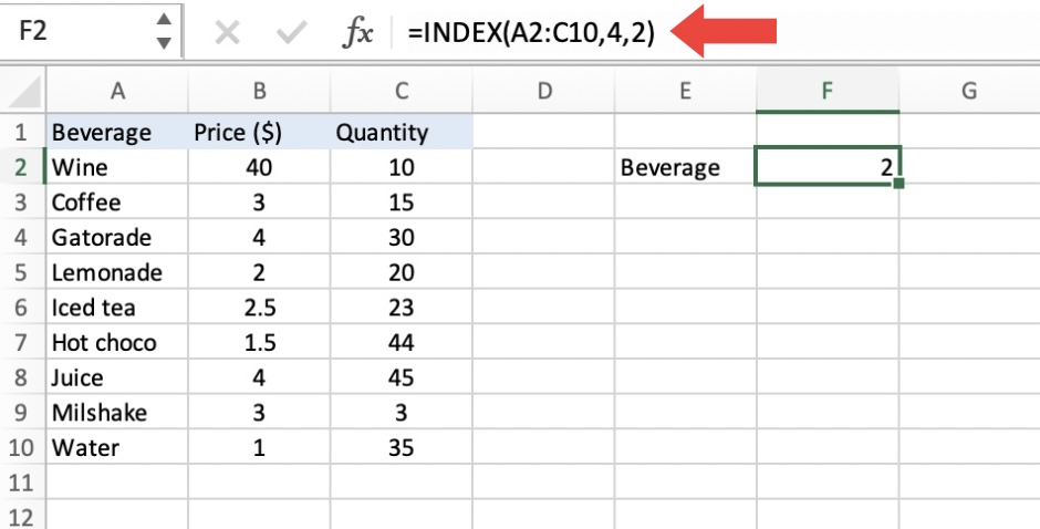
Suppose you want to retrieve the price of the Lemonade using the INDEX function. In this instance, you can specify both a row number and a column number while providing a larger range. The following INDEX formula utilizes the complete data range of A2:C10, with a row number of 4 and a column number of 2:
=INDEX(A2:C10,4,2)
Suppose you want to retrieve the price of the Lemonade using the INDEX function. In this instance, you can specify both a row number and a column number while providing a larger range. The following INDEX formula utilizes the complete data range of A2:C10, with a row number of 4 and a column number of 2, which corresponds to the price:
=INDEX(A2:A10,4)
In summary, the INDEX function retrieves a value at a specific location in a range of cells based on a numerical position. If the range is one-dimensional, a row number is adequate. If the range is two-dimensional, both the row and column numbers are required.
However, it is uncommon to know the position of data in a spreadsheet.
Thus, we require a mechanism to locate the positions of data we are seeking. This is where the MATCH function comes in handy.
The MATCH Function
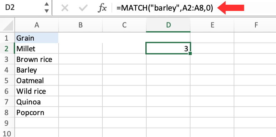
The MATCH function has a specific function: to determine the position of an item in a range of cells. For instance, you can use MATCH to locate the position of the word “barley” in a list of grains, like this:
=MATCH(“barley”,A2:A8,0)
As you can see, it does not matter if the range is vertical or horizontal:
It is crucial to note that the last argument in the MATCH function is match_type. This argument determines whether the matching should be exact or approximate. In most cases, you will want to use the value 0 to enforce exact match behavior. The match_type parameter defaults to 1, indicating approximate match, so it is important to specify a value to avoid any confusion.
INDEX and MATCH together
To combine the INDEX and MATCH functions in a single formula, you first need to understand that INDEX returns a value from a range based on a row and column number. Therefore, you can use MATCH to find the row or column number that you need to retrieve from the range.
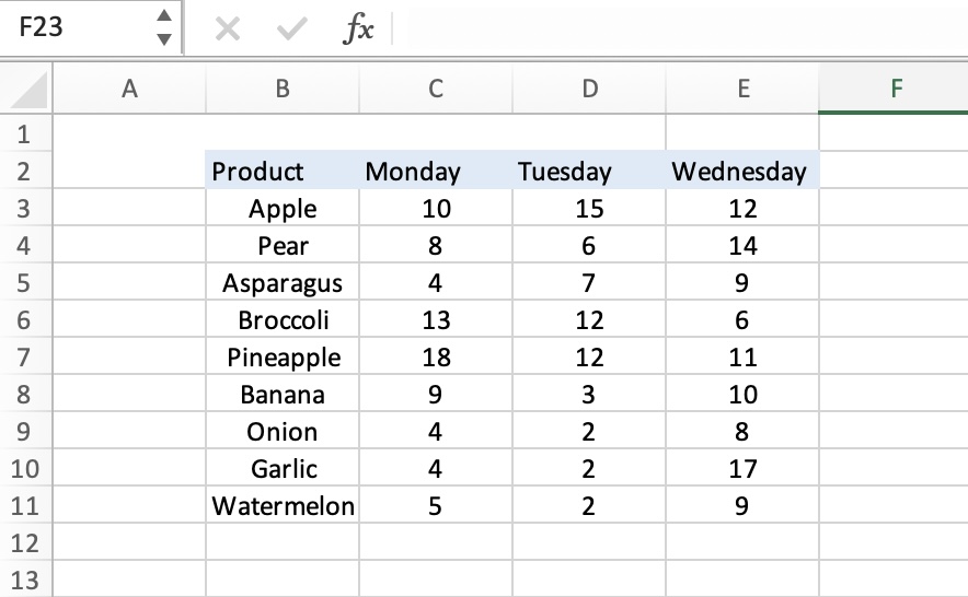
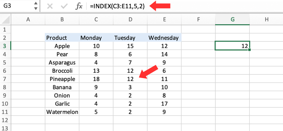
For example, consider the data below, which represents a table of produce and daily sales numbers for three days: Monday, Tuesday, and Wednesday.
Suppose we aim to create a formula that provides the sales number for Tuesday of a specific item. Based on our previous discussion, we are aware that we can provide INDEX with a row and column number to obtain a value. To illustrate, to obtain the Tuesday sales number for Pineapple, we need to specify the range C3:E11 with a row of 5 and a column of 2.
However, you don’t want to hardcode numbers. The dynamic lookup is the difference-maker.
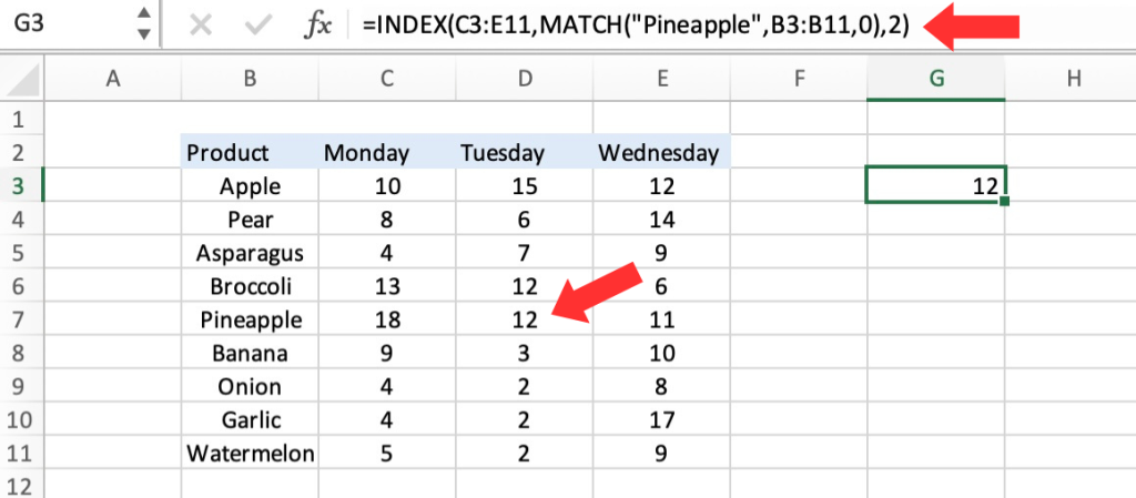
How can we achieve that? We can utilize the MATCH function, which is ideal for locating the positions we require. To begin, we can hardcode the column as 2 and make the row number adaptable by using MATCH. Here’s the updated formula, where the MATCH function is inserted inside INDEX in place of 5:
=INDEX(C3:E11,MATCH(“Pineapple”,B3:B11,0),2)
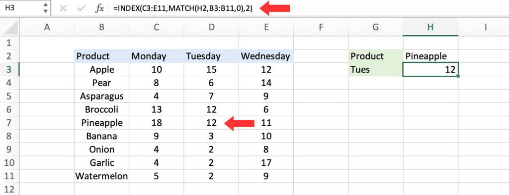
Taking things one step further, we’ll use the value from H2 in MATCH:
=INDEX(C3:E11,MATCH(H2,B3:B11,0),2)
In summary:
- INDEX needs numeric positions.
- MATCH locates those positions.
- MATCH is enclosed within INDEX.
Two-way lookup with INDEX and MATCH
In the previous example, we utilized the MATCH function to dynamically determine the row number, but the column number was hardcoded. Is there a way to create a completely flexible formula that can return data for any product in any day? To achieve this, we need to use MATCH twice: one to determine the row position and the other to determine the column position.
Based on the examples provided, it is evident that MATCH works effectively with arrays in both horizontal and vertical orientations. This implies that locating the position of a specified month using MATCH is a simple task. To illustrate, the following formula identifies the position of Wednesday, which is 3:
=MATCH(“Wednesday”, C2:E2,0) // returns 3
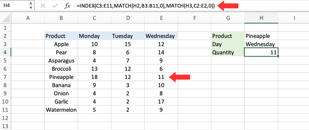
Naturally, it is preferable not to hardcode values. Therefore, let us modify the worksheet to enable the input of a day’s name and utilize MATCH to locate the relevant column number:
=INDEX(C3:E11,MATCH(H2,B3:B11,0),MATCH(H3,C2:E2,0))
After the initial MATCH formula returns 5 to INDEX as the row number, and the second MATCH formula returns 3 to INDEX as the column number, the formula is simplified to:
=INDEX(C3:E11,5,3)
and INDEX correctly returns 11, the quantity of Pineapples sold on Wednesday.
Left Lookup
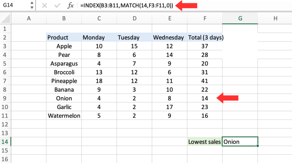
INDEX and MATCH offer a significant advantage over the VLOOKUP function, which is the capability to perform a “left lookup.” Essentially, this refers to a search in which the identifier column is located to the right of the values that require retrieval:
=INDEX(B3:B11,MATCH(14,F3:F11,0))
We can easily find out the onion’s total sales by using the VLOOKUP function. The left LOOKUP is the opposite of that. If we wanted to find out which product got the lowest amount of sales (14), it would lead to the onion.
Case-sensitive Lookup
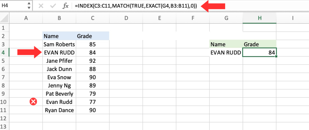
Although the MATCH function does not consider the case sensitivity, you can incorporate the EXACT function along with INDEX and MATCH to carry out a lookup that takes into account the upper and lower case, as demonstrated below:
=INDEX(C3:C11,MATCH(TRUE,EXACT(G4,B3:B11),0))
There you have it! In this article, we have covered how to use the INDEX and MATCH functions in Microsoft Excel, as well as a few others. As you can see, these lookup tools can be quite powerful in the right setting!
John Michaloudis is a former accountant and finance analyst at General Electric, a Microsoft MVP since 2020, an Amazon #1 bestselling author of 4 Microsoft Excel books and teacher of Microsoft Excel & Office over at his flagship Academy Online Course.

