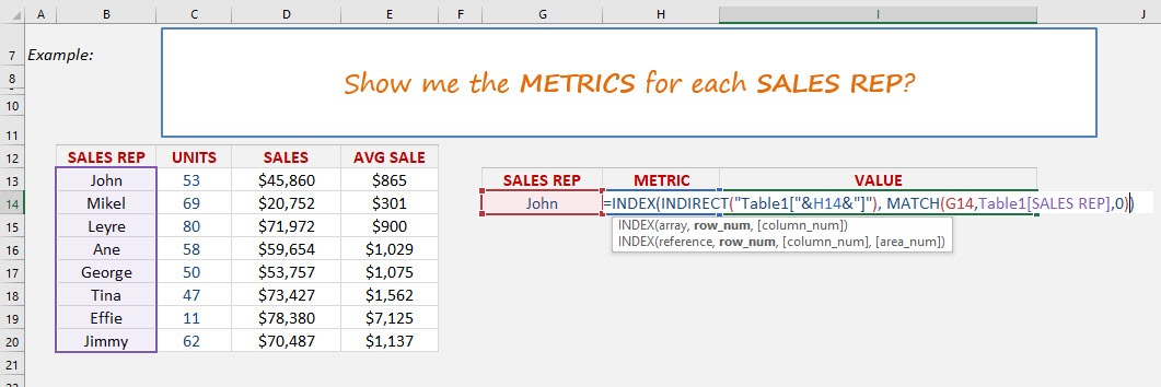
What does it do?
Searches the row position of a value/text in one column (using the MATCH function) and returns the value/text in the same row position from another column to the left or right (using the INDEX function)
Formula breakdown:
=INDEX(array, MATCH(lookup_value, lookup_array, [match_type])
What it means:
=INDEX(return the value/text, MATCH(from the row position of this value/text))
We can use the INDEX-MATCH formula and combine it with Data Validation drop down menus to return a value based on 2 criteria.
This is a little advanced so you will need to drop what you are doing and really focus. Let’s go…
First we need to convert our data into an Excel Table by pressing Ctrl+T
See tutorial on how to convert to an Excel Table here
We then create drop down menus for our Sales Rep column and another one for our Units/Sales/Avg Sale column names
See tutorial on how to insert drop down menus here
Once the above are done we need to create our formula.
Download the workbook below to practice this method.
STEP 1: We need to nest an INDIRECT function within the INDEX function and reference the Metric cell name (H14) with our Table name (Table1):
=INDEX(INDIRECT(“Table1[“&H14&”]”),
This will give us our dynamic column name within the Excel Table.
STEP 2: We need to lookup our Sales Rep within the Sales Rep column table:
=INDEX(INDIRECT(“Table1[“&H14&”]”),
Table of Contents
MATCH(G14,Table1[SALES REP],0))
So by combining these formulas we can choose two criteria (Sales Rep & Metric name) to return the respective value.
How to Index Match 2 Criteria with Data Validation in Excel
John Michaloudis is a former accountant and finance analyst at General Electric, a Microsoft MVP since 2020, an Amazon #1 bestselling author of 4 Microsoft Excel books and teacher of Microsoft Excel & Office over at his flagship Academy Online Course.


