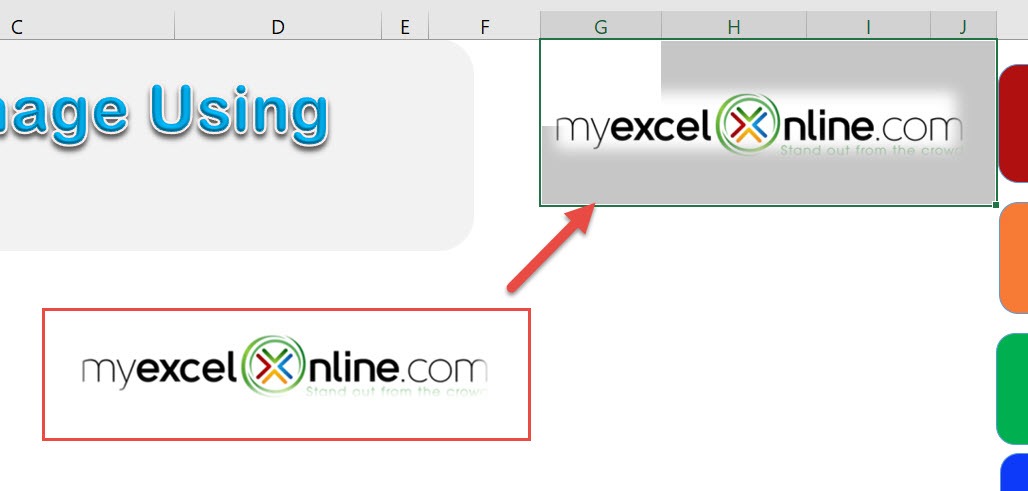
Did you know that you can create a linked image in Excel? It’s a cool feature if you that you can use to create dashboards wherein it is easier to resize images, then link them to the actual report. Let us use Excel Macros to create our own linked image!
Make sure your Excel has the Developer Tab enabled following this tutorial.
I explain how you can do this below step by step!
What does it do?
Creates a linked image based on your selection
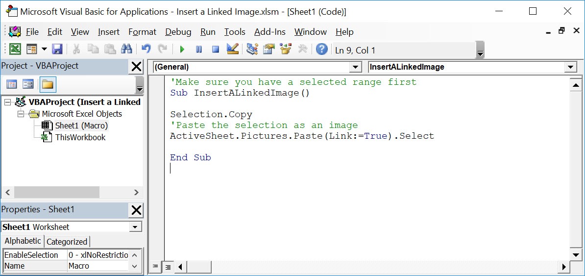
Copy Source Code:
'Make sure you have a selected range first
Sub InsertALinkedImage()

Selection.Copy
'Paste the selection as an image
ActiveSheet.Pictures.Paste(Link:=True).Select

End Sub
Final Result:
Exercise Workbook:
Let us try creating a linked image based on the logo. You can do this on any part of the spreadsheet!
STEP 1: Go to Developer > Code > Visual Basic
STEP 2: Paste in your code and Select Save. Close the window afterwards.
STEP 3: Let us test it out!
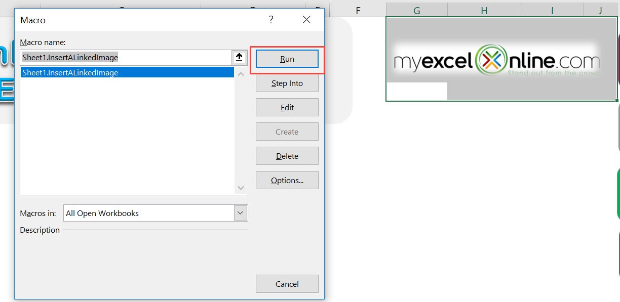
Open the sheet containing our target. Go to Developer > Code > Macros
Make sure the logo cells and your macro are selected. Click Run.
With just one click, you have created a linked image! Double click on it and it will highlight the logo!
How to Insert a Linked Image Using Macros In Excel
Bryan
Bryan is a best-selling book author of the 101 Excel Series paperback books.


