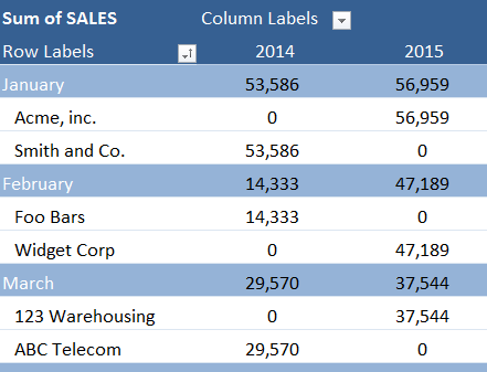
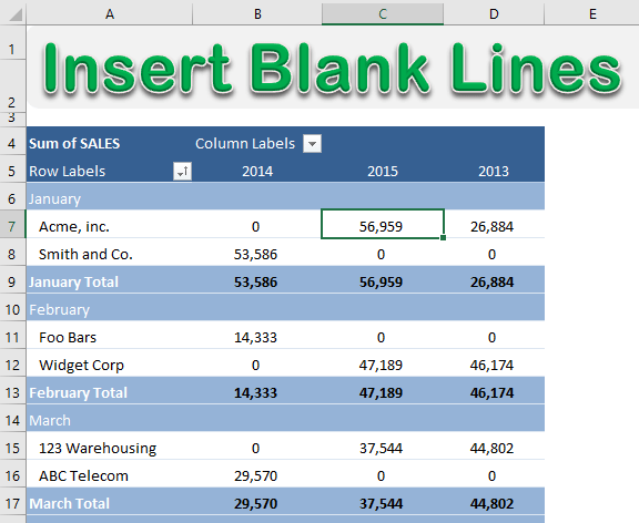
Pivot Table reports are shown in a Compact Layout format as a default and if you have two or more Items in the Row Labels (e.g.Month & Customer), then the Pivot Table report can look very clunky…
There is a cool little trick that most Excel users do not know about that adds a blank row after each item, making the Pivot Table report look more appealing.
Here is how to insert a row in Pivot Table!
Follow a step-by-step tutorial on how to insert row in pivot table and download this workbook to move along with us:
download excel workbookInsert-Blank-Lines.xlsx
STEP 1: Click any cell in the Pivot Table
STEP 2: Go to Design > Blank Rows
STEP 3: You will need to click on the Blank Rows button and select Insert Blank Line After Each Item
NB: For this to work you will need at least two Pivot Table Items in the Rows Labels
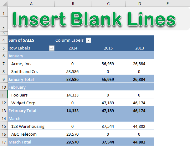
You then get the following Pivot Table report:
This tutorial shows you how to insert rows in pivot table and will make the Pivot Table look clean and more appealing.
You can easily remove this blank row from Pivot Table as well!
METHOD 1: Simply press CTRL + Z if you have recently inserted a blank row.
METHOD 2: Go to Design > Blank Row dropdown > Select Remove Blank Line After Each Item.
This will remove the blank rows after each item!
Using the Design Tab, you can easily insert blank row in pivot table or remove it!
Further Learning:
- How To Fill Blank Cells in Pivot Table
- Delete Blank Worksheets Using Macros In Excel
- ISBLANK Formula in Excel
HELPFUL RESOURCE:
Make sure to download our FREE PDF on the 333 Excel keyboard Shortcuts here:
John Michaloudis is a former accountant and finance analyst at General Electric, a Microsoft MVP since 2020, an Amazon #1 bestselling author of 4 Microsoft Excel books and teacher of Microsoft Excel & Office over at his flagship Academy Online Course.


