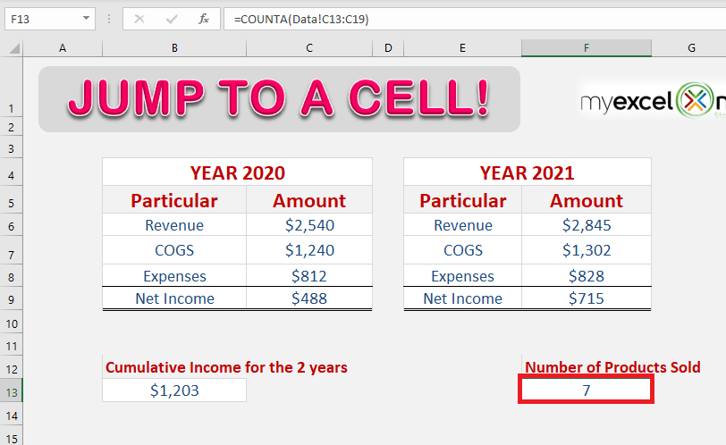
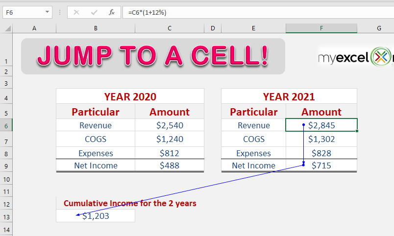
Ever encountered a situation when you are working on a spreadsheet created by someone else? Not sure about the cells being referred to in the formula?
When writing, editing, or auditing Excel formulas you will have to view and access the referenced cells within a formula argument.
There is a cool tip where you can jump to the referenced cell or range within the formula and make your changes.
Excel go to cell in formula is helpful if you want to check how the formula works or to make any changes to the formula.
Go To Functionality
Follow the step-by-step tutorial on Excel formula to go to a specific cell with an Excel worksheet to practice along:
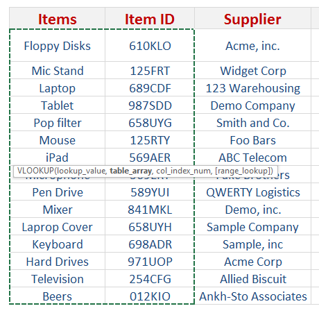
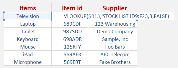
STEP 1: Double click inside your Excel formula
STEP 2: Select the formula argument that you want to edit with your mouse
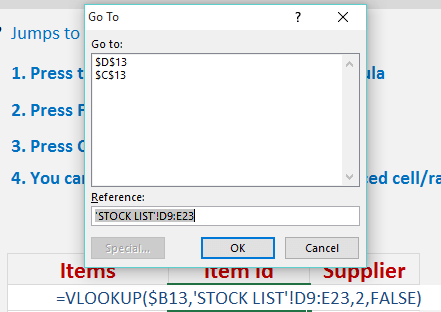
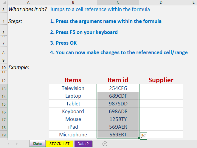
STEP 3: Press F5 which will bring up the Go To dialogue box and press OK
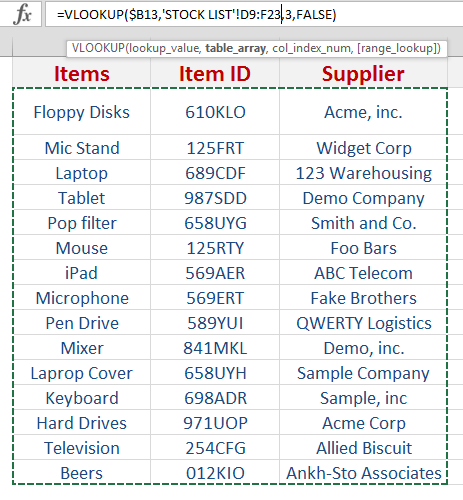
STEP 4: This will take you to the referenced cell/range
STEP 5: You can select the new range with your mouse and also make any changes to the formula bar
STEP 6: Press Enter and your formula is updated
This is how you can use the go to cell in Excel!
You can even use a simpler technique to Excel jump to cell in formula using Trace Dependents and Trace Precedents in Excel.
Let’s look at these two features in detail!
Trace Precedents
Precedent cells are the cells that are referred to by a formula.
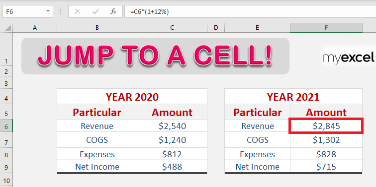
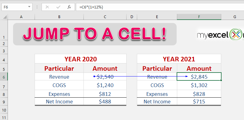
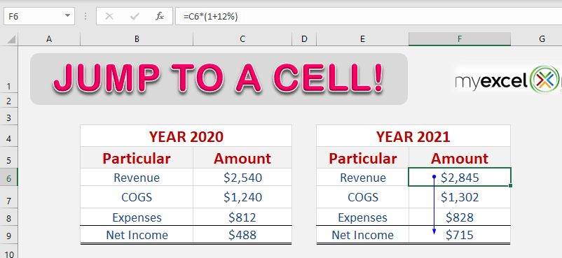
In the example below, cell F6 contains a formula that is getting value from another cell. You can use the Trace Precedents to take you to the cell from which you are getting the value.
Let’s see it can be done!
STEP 1: Select the cell F6.
STEP 2: Go to Formulas > Trace Precedents.
This will create arrows on your sheet that will indicate which cells affect the value of the currently selected cell.
To remove these arrows, Go to Formulas > Remove Arrows.
You can even use a keyboard shortcut to highlight the precedent cells.
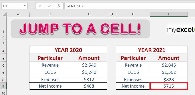
STEP 1: Select the cell F9.
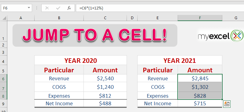
STEP 2: Press Ctrl + [. This will highlight all the cells mentioned in the formula.
You can press Tab to move between these cells.
Another cool tip is that this feature also works when the formula contains a link to an external workbook and that workbook is closed. When you press Ctrl + [, it will open the closed workbook and take you to that specific cell.
Let’s look at another example for this.
STEP 1: Select a cell that contains a formula linked to a different worksheet or an external workbook.
STEP 2: Go to Formulas > Trace Precedents.
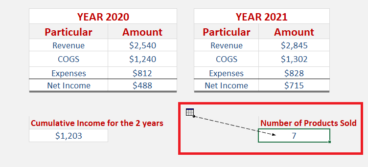
Since the dependent cells are placed in a different worksheet, it will be indicated with a black dash line and arrowhead pointed to a small picture.
STEP 3: Double click on the dashed line to open the dialog box that lists the dependent cells.
STEP 4: Select the cell from the list and press OK. Excel will take you to the referred cell.
Trace Dependents
Dependent cells can be used to show the cells that are affected by the active cells. To see the cells that are dependent on the active cells, follow the steps below:
STEP 1: Select the cell you want to analyze.
STEP 2: Go to Formulas > Trace Dependents or Press Ctrl +].
This will highlight the dependent cell with blue arrows.
STEP 3: Click on Trace Dependents again to show more cells that are related to the active cells.
Further Learning:
- How to Apply Formula to Entire Column in Excel
- How to Master Excel Formulas – The Ultimate Guide
- Why Excel Formula giving Wrong Answers?
Make sure to download our FREE PDF on the 333 Excel keyboard Shortcuts here:
John Michaloudis is a former accountant and finance analyst at General Electric, a Microsoft MVP since 2020, an Amazon #1 bestselling author of 4 Microsoft Excel books and teacher of Microsoft Excel & Office over at his flagship Academy Online Course.


