When working with datasets in Microsoft Excel that require the extraction of the largest values based on specific conditions, the regular LARGE function might fall short as it cannot filter data by criteria. However, by combining the LARGE function with the IF function in an array formula, you can create customized ‘LARGE IF’ formulas to find top values that meet single or multiple criteria—effectively bridging the functionality gap and providing precise, condition-based results.
Key Takeaways
- The Excel LARGE IF formula does not exist by default, but you can create one by nesting IF functions within the LARGE function to find large numbers based on criteria.
- To retrieve the nth largest value with a single criterion, combine the LARGE function with an IF statement specifying the condition to meet.
- For multiple criteria, you can extend the IF function with the use of and/or operator to test multiple criteria.
- This method allows users to filter and analyze large datasets, extracting specific high-value data points according to defined single or multiple conditions.
Download the workbook and follow along with the tutorial on how to use large if formulas in Excel – Download excel workbookLarge-IF-Formula-in-Excel.xlsx
Table of Contents
Harnessing the Power of Excel for Advanced Data Analysis
The Vital Role of LARGE IF Formulas in Excel
In today’s data-driven environment, Microsoft Excel remains an indispensable tool for performing complex data analysis. Among Excel’s arsenal of functions, the LARGE IF combination plays a crucial role. Unfortunately, Excel doesn’t have a built-in LARGE IF function, but savvy users have developed a way to emulate this functionality by combining the LARGE function with the IF function to filter and analyze data based on specific conditions.
Understanding the Mechanics of LARGE and IF Functions
Before delving into the LARGE IF formula, it’s important to understand the basics of the LARGE and IF functions individually, as they are the building blocks of the combinatorial formula.
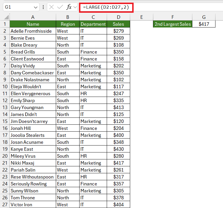
The LARGE function in Excel is designed to return the n-th largest value from a data set. For example, =LARGE(range, k) will give you the k-th largest value within the specified range.
This formula will provide you with the 2nd largest sales –
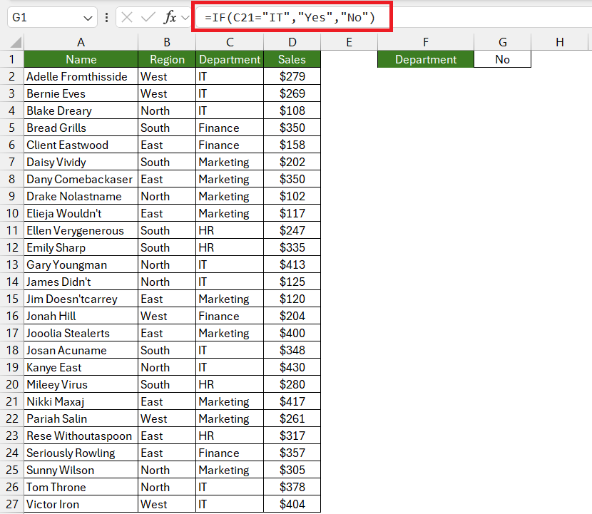
On the other hand, the IF function is used to conduct logical tests and returns values based on whether the test is true or false. Its syntax is =IF(condition, value_if_true, value_if_false).
If the department is IT, then the result displayed will be “Yes” or else it will be “No”.
When we intertwine these two functions, we provide a powerful way to extract significant numbers based on specific criteria, enabling dynamic and condition-based analysis. Let’s break down the functions individually and then see how they work together.
Crafting Dynamic Data Solutions with LARGE IF
Example 1: LARGE IF with One Criteria
The basic LARGE IF formula combines the LARGE and IF functions to apply a single criterion to a dataset and retrieve the n-th largest value that meets that condition. Applying the LARGE IF formula to a dataset when you need to specify a single criterion is straightforward. Here’s an example to illustrate:
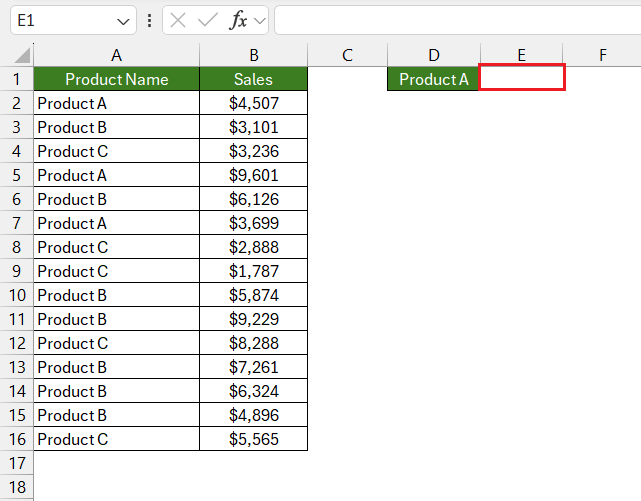
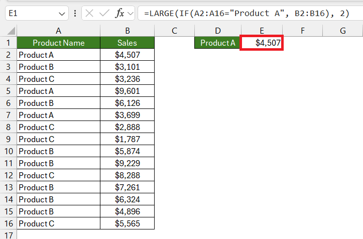
Scenario: Suppose you have a list of sales figures for multiple products, and you want to find the second-largest sales figure specifically for product “A”.
Dataset Layout:
- Column A contains product names (A2:A16).
- Column B holds the sales figures (B2:B16).
Objective: To find the 2nd largest sales figure for product “A”.
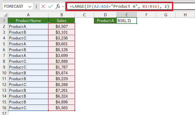
Formula:
This formula IF(A2:A16="Product A", B2:B16) filters the sales figures by product “A”. The LARGE function then seeks the second-largest number within this specific subset.
Steps:
STEP 1: Choose a cell where you wish the result to be displayed.
STEP 2: Enter the formula =LARGE(IF(A2:A16="Product A", C2:C16), 2).
STEP 3: The result will display the second-largest sales figure for Product A.
By modifying the criteria and the k-th value, you can repurpose this basic formula for various single-condition data retrieval tasks. Remember to adjust your range and criteria to match your specific dataset when applying the formula.
Example 2: Filter n-th Largest Values Using Multiple AND Criteria
When the need arises to filter data using multiple criteria, the basic LARGE IF formula must be expanded. Let’s consider an example using AND logic where two conditions must be met simultaneously.
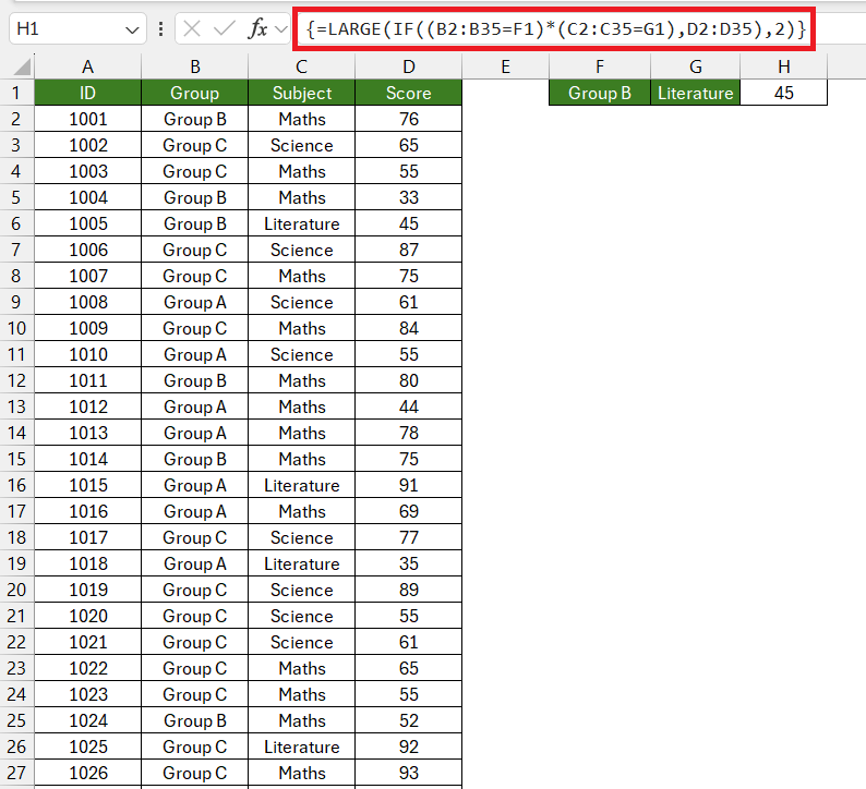
Scenario: Imagine you have the scores of students for different subjects, and you need to find the 2nd highest scores for the subject ‘Literature’ from ‘Group B’.
Dataset Layout:
- Column B contains group information (B2:B35).
- Column C contains subject names (C2:C35).
- Column D holds the scores (D2:D35).
Objective: Locate the 2nd highest Literature score from Group B.
Formula:
=LARGE(IF((B2:B35=F1)*(C2:C35=G1),D2:D35),2)
In this formula, (IF((B2:B35=F1)*(C2:C35=G1),D2:D35) uses the IF function to screen for scores where the corresponding rows in Column B are “B” (for Group B) and rows in Column C are “Literature” (for the subject). The multiplication sign (*) works as an AND operator here to ensure that both conditions must be true. LARGE acts on this filtered set to find the third-highest score.
The provided result will be the 3rd highest score for the subject Literature specifically within Group B. Altering the conditions and the n value in the LARGE function can adapt the formula to different scenarios and datasets.
By mastering this concept, you can effectively use Excel to analyze data with multiple conditional statements and extract valuable insights tailored to specific requirements.
Formula 3: Filter n-th Largest Value Using Multiple OR Criteria
In scenarios where you need to retrieve an n-th largest value based on one of the multiple potential criteria being met (OR logic), the combination of the LARGE and IF functions becomes even more versatile. Let’s walk through an example to clarify this.
Scenario: Continuing with the student scores database, let’s say this time you’re interested in finding the 3rd largest scores across both Literature or Maths subjects.
Objective: To retrieve the 3rd largest from either Literature or Maths.
Formula:
=LARGE(IF((C2:C35=F1)+(C2:C35=G1),D2:D35),3)
This complex formula uses an OR logic within the IF function, where (C2:C35=F1)+(C2:C35=G1) signifies that either subject condition being true will pass the filter.
With this approach, you’re capable of combining the power of LARGE and IF with the flexibility of OR logic, thus extending Excel’s functionality to accommodate complex and dynamic data analysis tasks.
Tips for Troubleshooting Common LARGE IF Errors
Why Your Excel LARGE IF Function Might Be Failing
If you’re struggling with the LARGE IF function not performing as expected, there could be several contributing factors. Here are some potential reasons why your LARGE IF function might be failing:
Array Formula Not Entered Correctly: Prior to Excel 365, LARGE IF is an array formula. If you do not enter it correctly with CTRL + SHIFT + ENTER, it may not work as intended.
Incorrect Range References: Mismatches in the range references for criteria and the values being evaluated can cause errors. Ensure that your ranges are aligned correctly.
Data Type Mismatch: The IF function can only test for values that are appropriately formatted for the conditions set. For instance, comparing text to numbers will result in an error.
Not Using Absolute Cell References Where Needed: If your formula includes references that are not fixed (absolute) and it is copied across cells, the references will change, leading to incorrect results.
Incomplete Criteria: If your logical criteria are not fully specified or have typos, the IF function won’t be able to process them, and the LARGE function will not return the correct value.
Nesting Too Many IF Functions: Excel has limitations on how many nested functions can be used. Exceeding this can cause the formula to break down.
Lack of Required Data: If the k value specified in the LARGE function is greater than the number of values that meet the IF condition, the formula will result in an error.
Formula Evaluation Errors: Errors can creep in if the formula is misconstructed – using incorrect syntax such as missing commas, parentheses, or using the wrong operators.
By troubleshooting these common issues, you’ll often be able to identify why your LARGE IF function isn’t working correctly and make the necessary adjustments to get it back on track.
FAQ: Expert Answers to Your LARGE IF Questions
How can I combine LARGE IF with other functions for more complex analyses?
You can combine the LARGE IF function with other Excel functions such as SUM, AVERAGE, or COUNT to conduct more sophisticated analyses. By nesting these functions within the parameters of a LARGE IF array formula, you can perform conditional analysis based on multiple criteria.
What are the limitations of the LARGE IF function and how can I work around them?
The LARGE IF function may pose challenges with data quality, as inaccuracies like outliers or missing values can skew results, and handling duplicated values requires caution to avoid unexpected outcomes. To work around these limitations, ensure data sets are clean and consistent, manage duplicates wisely, and for large-scale analysis, optimize formulas or consider alternative methods to prevent performance lag. Moreover, supplement the LARGE function with other statistical tools and visualizations for a well-rounded analysis.
How to do a large if formula in Excel?
To perform a LARGE IF formula in Excel, you can combine the LARGE and IF functions into an array formula. For a single criterion, use the formula `=LARGE(IF(range=criteria, return_range), k)’, replacing `range`, `return_range`, `criteria`, and `k` with your specific data. Remember to press CTRL + SHIFT + ENTER to input the array formula correctly in Excel versions 2019 and earlier.
How to find and get the largest value based on multiple criteria in Excel?
To find and get the largest value in Excel based on multiple criteria, use the formula `{=LARGE(IF((criteria1)*(criteria2), value_range), n)}` where “criteria1” and “criteria2” are the conditions that must be met, “value_range” is the range containing the numeric values, and “n” specifies the nth largest value you wish to return. Remember to press `Ctrl + Shift + Enter` after typing the formula to enter it as an array formula. If relevant, you can extend the formula to include additional criteria by multiplying them within the IF function.
John Michaloudis is a former accountant and finance analyst at General Electric, a Microsoft MVP since 2020, an Amazon #1 bestselling author of 4 Microsoft Excel books and teacher of Microsoft Excel & Office over at his flagship Academy Online Course.
