In this blog, you will learn two methods on how to lock formula cells in Excel.
In Excel, you can easily create and edit formulas using the formula bar or double-clicking the cell itself.
But, Every light has its shadow.
Because it is that easy to edit a formula, you can accidentally enter the delete button or make any unwanted change in a formula. This may lead to errors that may be difficult to spot later.
So, it is important to know how to lock formula cells in Excel!
There may be situations when you have to share these files with a colleague or boss. At those times, hiding or protecting the formula will become of utmost importance.
Two methods on how to protect formula cells in Excel are:
Let’s look at each of these methods!
Locking the Cells
If you have a workbook with lots of formulas and you want to protect those formulas from being amended by other people who share your workbook, then you can even lock the cells!
Watch it on YouTube and give it a thumbs-up!
You need to follow these steps on how to lock formula cells in Excel and download the Excel Workbook below to practice along with:
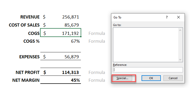
STEP 1: Press the Go To Special shortcut CTRL+G.
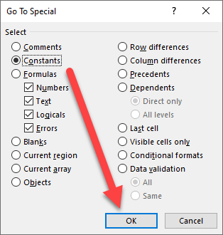
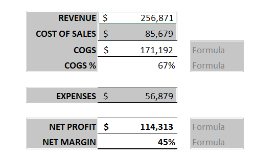
STEP 2: Select the Constants box and press OK (this highlights all the non-formula cells)
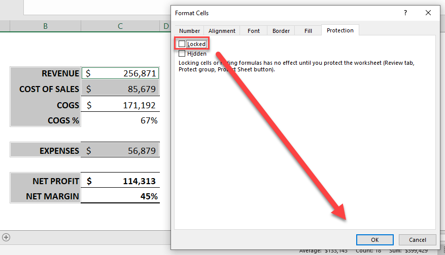
By default, all the cells in Excel are locked. So, we need to select the cells containing constant values and unlock them.
In the end, only the cells containing formulas will remain locked!
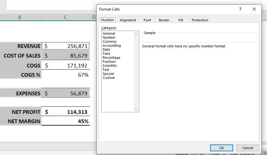
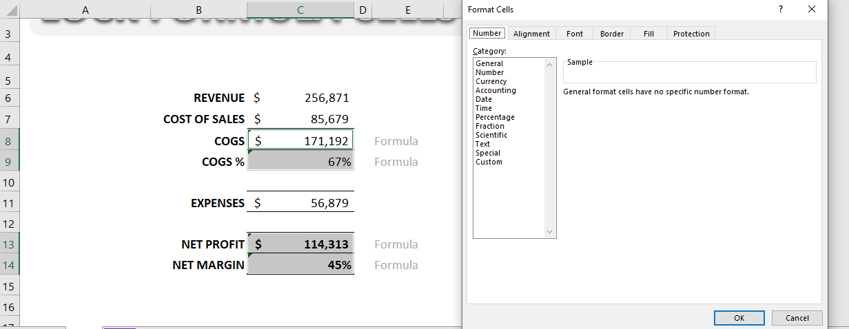
STEP 3: Press CTRL+1 to bring up the Format Cells dialogue box
STEP 4: Select the Protection tab and Un-check the Locked box
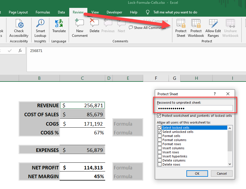
STEP 5: In the menu ribbon go to Review > Protect Sheet > then enter your custom password (optional)
This will lock all the cells that are not constant, so all the formula cells 🙂
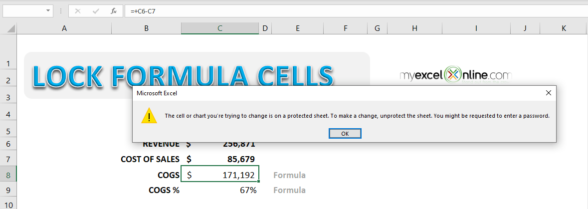
Now, if you try to make any change in the protected cells you will be prompted with this message and will not be able to make any edits.
This is how to protect formulas in Excel by locking the cells.
In this method, even though the cells will be locked you can still see the formula used.
To hide the formula from others, follow the second method.
Hiding the Formula Bar
An easy way to prevent a user from making an undesired change in a cell, you can hide the formula in the formula bar. Follow the steps below to do so:
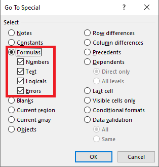
STEP 1: Press the Go To Special shortcut CTRL+G.
STEP 2: Select the Formulas box and press OK (this highlights all the formula cells)
STEP 3: Press CTRL+1 to bring up the Format Cells dialogue box.
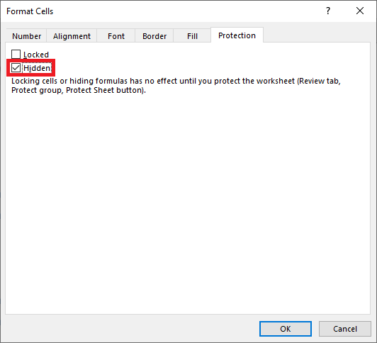
STEP 4: In the Format Cells dialogue box, go to the Protection tab and un-check the Locked box, and check the Hidden box.
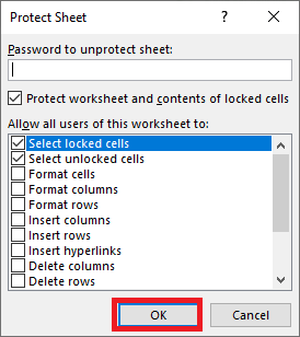
STEP 5: Go to the Review Tab > Protect Sheet.
STEP 6: In the Protect Sheet dialog box, Click OK.
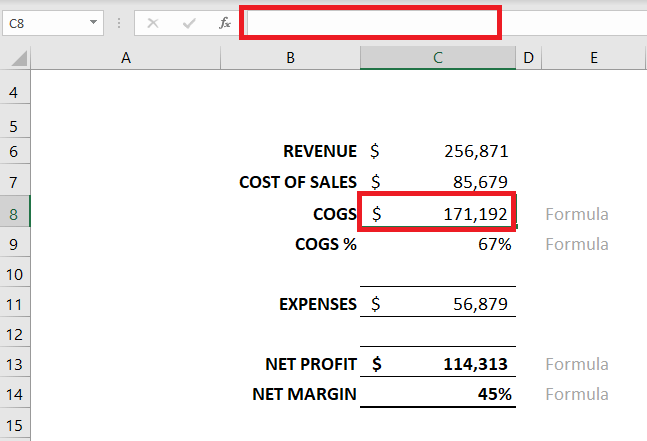
STEP 7: Select the cell C8, you will see that the formula bar is blank!
It is important to understand that the sheet needs to be protected in order to hide the formula. Simply checking the hidden box will not do the trick!
This completes our tutorial on how to protect formula in Excel!
Conclusion
If you have sensitive data in your Excel workbook that you wish to hide from others using the file, you can follow one of these two methods on how to lock formula cells in Excel.
You can even use these methods to simply protect your workbook from any unwanted and accidental change being made.
In the first method, you can prevent others from making any changes to the cells with formulas by locking the cells.
But the formula used in the cell would still be visible in the formula bar
You can follow the second method in which the formula in the cell will not be visible in the formula bar as well.
HELPFUL RESOURCE:
Make sure to download our FREE PDF on the 333 Excel keyboard Shortcuts here:
John Michaloudis is a former accountant and finance analyst at General Electric, a Microsoft MVP since 2020, an Amazon #1 bestselling author of 4 Microsoft Excel books and teacher of Microsoft Excel & Office over at his flagship Academy Online Course.

