Sometimes when you are sharing an Excel Pivot Table with your colleagues you do not want the other user(s) to mess with your Pivot Table layout and format.
What you can do is learn how to lock pivot table and only allow the user(s) to select the Slicers, making your report interactive and secure from Excel novices like your boss 🙂
Here is a step-by-step tutorial on How to Lock Pivot Table but not the Slicers:
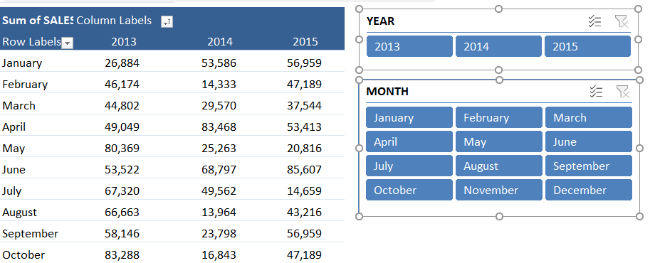
STEP 1: Click on a Slicer, hold the CTRL-key and select the other Slicers.
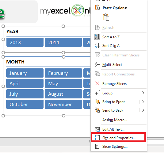
STEP 2: Right-click on a Slicer and select Size & Properties.
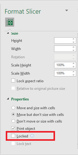
STEP 3: In the Format Slicer dialog box, Select Properties, “uncheck” the Locked box.
STEP 4: Go to the ribbon menu and select Review > Protect Sheet.
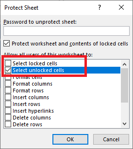
STEP 5: “Uncheck” the Select Locked Cells and “Check” the Select Unlocked Cells.
STEP 6: Enter a password (optional) and press OK.
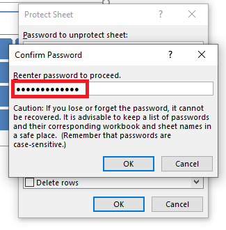
STEP 7: Re-enter the password and press OK.
Download workbook – unlocked Lock-the-workbook-Unlocked.xlsx
Download workbook – lockedLock-the-workbook-Locked.xlsx (Password to unlock: myexcelonline)
This completes the tutorial on how to lock pivot table format and how to lock slicers in Excel!
Further Learning:
- Unleashing the Power of Pivot Tables in Excel – A Practical Guide
- Select & Format Fields in Excel Pivot Tables
- Customising Excel Pivot Table Styles
INSPIRED FROM THIS ONLINE COURSE:
John Michaloudis is a former accountant and finance analyst at General Electric, a Microsoft MVP since 2020, an Amazon #1 bestselling author of 4 Microsoft Excel books and teacher of Microsoft Excel & Office over at his flagship Academy Online Course.
