What does it do?
Looks up a value from a table array or one-row / one-column range
Formula breakdown:
=LOOKUP(lookup_value, lookup_vector, [result_vector])
What it means:
=LOOKUP(value to be approximately matched, range of values to be matched against, [the matching value to be displayed])
Have you ever tried getting approximate matches in Excel? Approximate matches are used when you have an ascending table like Commission Bonus Rates or Income Tax Rates.
If you have tried out Vlookup Approximate Match in Excel, there is another cool way to do this! You can use the LOOKUP Formula to accomplish this as well.
IMPORTANT: For the LOOKUP Approximate Match to work in Excel, the lookup_vector has to be sorted in ascending order!
So the way that this formula works is that it looks at the first value in the lookup_vector that is greater than the lookup_value and then goes back one value. If a result_vector is provided, then the LOOKUP Formula will get the result from there, otherwise it simply gets it from the lookup_vector.
I explain how you can do this below:
STEP 1: We need to enter the LOOKUP function in a blank cell:
=LOOKUP(
STEP 2: The LOOKUP arguments:
Table of Contents
lookup_value
What is the value to be approximately matched?
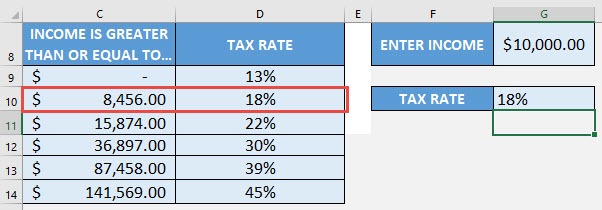
Select the cell containing the value. In our case, it is the $10,000 income:
=LOOKUP(G8,
lookup_vector
Where is the range of values to be matched against?
Now we need to select the range that contains the income values. It should be sorted in ascending order for the LOOKUP Formula to work.
=LOOKUP(G8, C9:C14,
result_vector
Where is the range of values to contains the value to be displayed as the final result?
Now we need to select the range that contains the tax rates. This is what we want to display as our final result of the lookup.
=LOOKUP(G8, C9:C14, D9:D14)
It was able to find out that the tax rate is 18%!
How to Use the LOOKUP Formula in Excel
Bryan
Bryan is a best-selling book author of the 101 Excel Series paperback books.


