When working with large datasets in Microsoft Excel, it often becomes necessary to retrieve information efficiently. A common task is to lookup row and extract an entire row based on a specific criterion. This can be accomplished by employing the versatile combination of the INDEX and MATCH functions or using the newer XLOOKUP function.
Through this tutorial, we will explore the method of utilizing these functions to effectively perform lookup row in Excel, greatly simplifying data analysis and organization tasks.
Key Takeaways
- The XLOOKUP function simplifies the process of retrieving an entire row by defining the lookup value, the lookup array, and the return array.
- For ranges not utilizing XLOOKUP, the INDEX and MATCH functions can be combined to perform a row lookup by matching the lookup value with its position and returning the corresponding row.
- Lookup functions can be integrated within other Excel functions such as SUMIF, CONCATENATE, MIN, and AVERAGE to perform calculations on the retrieved row data.
- The FILTER function also offers a solution for row lookups, providing an alternative method when specific conditions or criteria need to be met.
Download the Excel Workbook and follow the tutorial on how to lookup row in Excel – Download excel workbookLookup-Row-in-Excel.xlsx
Overview of Row Lookup in Excel
In the realm of Excel, a row lookup involves finding a specific set of data across a table‘s row based on given criteria. This often means you are taking a key value and using it to find an entire set of related data in that row. It’s like having a nifty treasure map where ‘X’ marks the spot, except in this case, ‘X’ is your lookup value and the treasure is the data you retrieve!
The Essentials for Mastering Lookups
When diving into the world of Excel lookups, mastering a few key concepts and functions will transform you into a lookup wizard. Firstly, understand that the lookup value is your starting point — this is what Excel searches for within your dataset. Then there’s the lookup array, where Excel scours through to find a match for your lookup value.
Next up, familiarize yourself with vital functions such as VLOOKUP or its more flexible counterparts, INDEX and MATCH, and the newer, more powerful XLOOKUP. Each plays a critical role, with INDEX and MATCH joining forces to accurately pinpoint data, and XLOOKUP bringing ease and enhanced functionality to the table. Remember, practice is key, so don’t shy away from experimenting with these functions to see how they can best serve your data needs.
Table of Contents
Simplifying Your Spreadsheets: Key Functions Explained
The Role of VLOOKUP in Row Fetching
VLOOKUP stands for Vertical Lookup, and it’s a go-to for many Excel users when they need to retrieve information from a specific row in a dataset. This function searches for a value in the first column of a table and fetches the data in the same row from a column you specify. It’s quite the workhorse for simple row-fetching tasks!
Formula breakdown:
=VLOOKUP(lookup_value, table_array, col_index_num, [range_lookup])
However, while VLOOKUP is straightforward and widely used, it does have its limitations — it cannot look to its left, and it only fetches one cell value per row. For more complex tasks, you might need to upgrade to other methods, but for basic data retrieval, VLOOKUP remains a steadfast ally in the world of Excel.
Advancing with INDEX and MATCH
Moving beyond VLOOKUP, the dynamic duo of INDEX and MATCH functions steps in to offer a versatile and robust approach for lookup row in Excel. Their combined power lies in the ability to search through columns and rows flexibly, without the constraints of VLOOKUP’s column limitations.
Here’s how they work in tandem: MATCH is like the scout, seeking out the exact location of your desired data—the row number in this case. Then, INDEX assumes the role of the retriever, using the location provided by MATCH to grab the entire row of data you’re after. It’s a surefire method when dealing with more intricate tables or when your lookup value isn’t snugly situated in the first column.
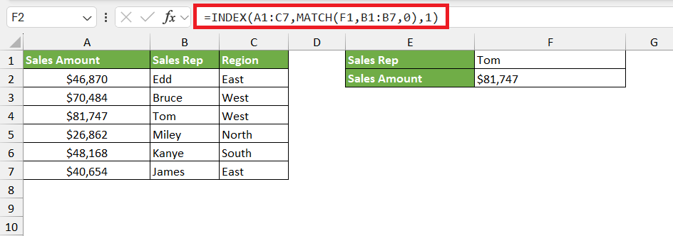
To fetch an entire row using INDEX and MATCH, you’d set up a formula like this:
=INDEX(data, MATCH(lookup_value, lookup_array, 0), 1)
This powerful pairing is essential for those seeking precision and flexibility in their Excel endeavors.
Enhancing Data Retrieval: Techniques and Examples
Use VLOOKUP to Return Entire Row in Excel
Diving into a practical scenario, let’s imagine you want to retrieve the entire row of data related to a specific product from a sales report spreadsheet using VLOOKUP. Here’s the way to make Excel do the heavy lifting for you:
To fetch the entire row data of a matched value, use this formula:
=VLOOKUP(lookup_value, table_array, {column reference}, FALSE)
In this formula:
lookup_valueis the identifier you’re using to find the related row, such as a product ID or name.table_arrayis the range of cells that contains the data.{column reference}is an array constant, for example{1,2,3,4,5}, which specifies that you want to return values from these columns of the array.FALSEinstructs Excel to find an exact match.
Enter the above formula into the first cell where you want the row data to appear, then drag the formula across the row to retrieve each column’s data of that matched value.
Remember, pressing Ctrl + Shift + Enter together converts this into an array formula for older Excel versions, which is essential for returning multiple columns simultaneously. In newer Excel versions, dynamic arrays handle this natively without special keystrokes.
Integrating LOOKUP with Other Important Excel Functions
Combining LOOKUP functions with other Excel stalwarts can create a powerhouse of data processing efficiency. When you integrate functions like IF, SUMIF, or CONCATENATE with LOOKUPs, you’re essentially choreographing a data ballet that effortlessly waltzes through large worksheets to find, calculate, and organize your numbers or text.
For example, you might use a VLOOKUP function to find a value, then nest it within an IF statement to categorize data based on the result.
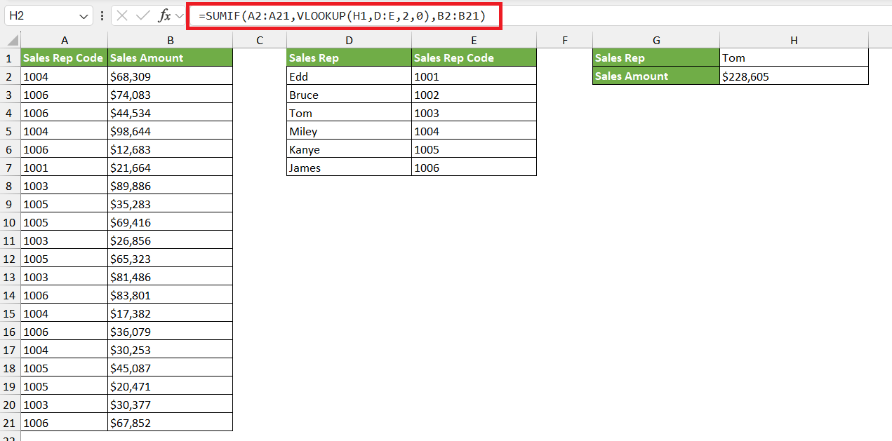
Or perhaps use VLOOKUP with SUMIF to tally totals only for rows that match certain criteria.
CONCATENATE can be used alongside VLOOKUP to merge data from the retrieved rows to create a new string of information.
These integrations are almost like Excel macros enabling you to construct customized formulas tailored to your data analysis requirements, saving time and enhancing accuracy.
By mastering these integration techniques, you guarantee that you have the right tool for virtually any Excel task you might encounter.
Practical Use Cases for Combining Multiple Criteria in Lookups
Excel’s ability to handle multiple criteria in lookups is a game-changer for in-depth data analysis. One might need to pull records where several conditions are met – think of finding the sales numbers for a specific product, in a certain region, during a designated time frame.
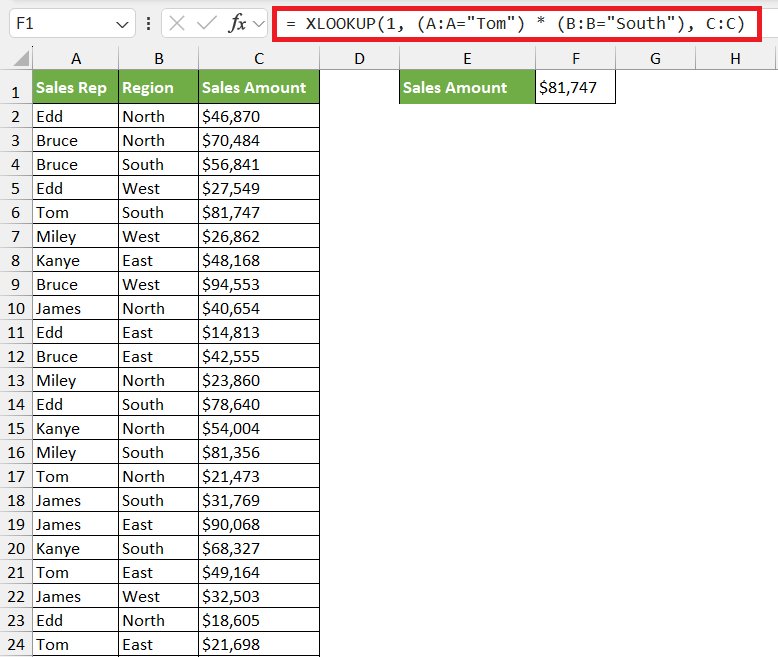
XLOOKUP, with its native array handling, shines here, allowing you to construct criteria using logical expressions. If you are seeking the first order to a city over a certain amount, for instance, you can create an array using conditions like so:
=XLOOKUP(1, (criteria_range1 = criteria1) * (criteria_range2 = criteria2), sum_range)
This effectively screens your dataset for multiple conditions, drastically reducing the time you spend on manually sorting through data.
Becoming adept at using Excel for multiple criteria lookups transforms complex tasks into simple operations, enabling you to handle large datasets with relative ease.
With FILTER: Dynamic Array Formulas for Modern Excel Versions
The FILTER function is a standout feature available in modern Excel versions, harnessing the power of dynamic array formulas. It’s designed to excel where you need to pull through multiple rows of data based on specific criteria with utmost efficiency. FILTER sifts through your data array and applies the criteria you define to return every row that matches.
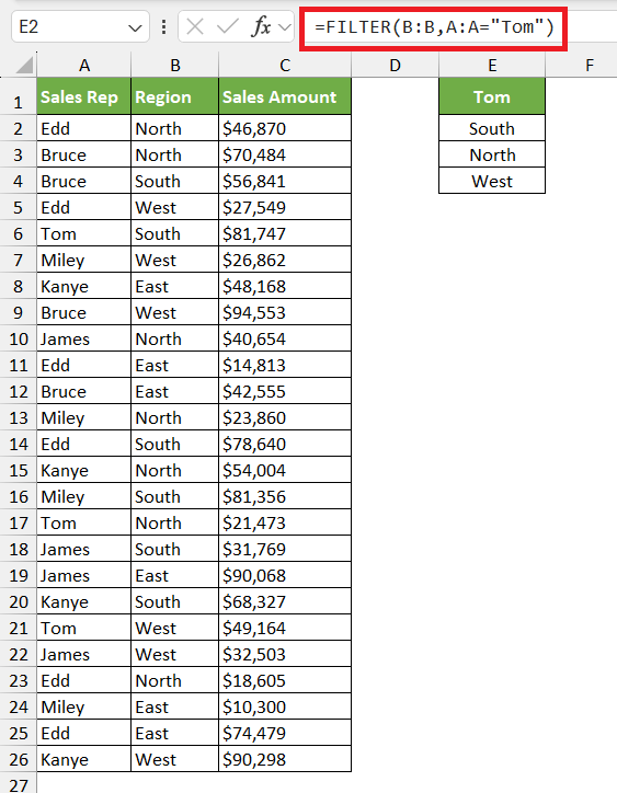
Imagine you have a list of sales representatives and want to display all the regions they are operating in. Your FILTER formula might look something like this:
=FILTER(region, sales rep=”Tom”)
Excel users who have upgraded to Microsoft 365 or Excel 2019 onward will find FILTER a transformative tool, facilitating a more fluid and dynamic approach to data analysis.
FILTER can replace many traditional lookup uses, especially when dealing with multiple criteria or the need for flexibility, marking a significant leap forward in Excel’s functional repertoire.
Navigating Potential Pitfalls: Tips and Troubleshooting
Common Issues When Looking Up Entire Rows and How to Solve Them
When attempting to look up entire rows in Excel, users often encounter a few common issues. One such challenge is when the VLOOKUP function doesn’t return the full row because it’s constrained to only return data from specific columns. An easy fix? Switch to INDEX and MATCH or XLOOKUP, which can handle entire rows by adjusting the return_array argument to cover the entire row range.
Another typical problem arises when there are duplicate values in your lookup column that cause the function to grab the first match only. You can tackle this by ensuring your search column contains unique values or by using the FILTER function in the latest versions of Excel which can return all matching instances.
Performance can also take a hit when you’re dealing with a massive dataset, leading to slow calculation times. To counteract this, consider converting your data range to an Excel table which can speed up the processing of lookups, or break the data into smaller chunks.
When it comes to errors like #N/A, which means no match was found, you can utilize the IFERROR function to provide an alternative result or a simple message like “Not Found”, making your worksheet cleaner and more user-friendly.
By staying vigilant about these potential pitfalls and knowing how to resolve them, you maintain the integrity of your data analysis and save yourself from unnecessary headaches.
Performance Tips for Large and Complex Datasets
Handling large and complex datasets in Excel requires a thoughtful approach to maintain performance and speed. Here are some expert tips to keep Excel running swiftly:
- Opt for INDEX-MATCH or XLOOKUP over VLOOKUP, as they can be more efficient, especially when working with large tables.
- When possible, use Excel Tables (Ctrl + T) as they’re optimized for performance and can make your lookup formulas easier to manage and understand.
- Consider using the FILTER function or dynamic arrays, which handle large datasets more efficiently in the newer versions of Excel.
- Keep your lookup arrays short by limiting the range to the necessary rows and columns, avoiding whole column references like A:A.
- If you’re using array formulas, press
Ctrl+Shift+Enteronly when needed, as they can be processor-intensive. - Regularly clean and organize your data to remove any unnecessary calculations or formatting which can slow down Excel.
By implementing these strategies, you can streamline your workbook’s performance, making data retrieval a breeze, even with the most daunting of datasets.
FAQ: Expert Answers to Common Lookup Queries
How to do a lookup row in Excel?
To do a lookup row in Excel, you can combine the INDEX and MATCH functions: =INDEX(array, MATCH(lookup_value, your_row_range, 0),column_num). This retrieves the value that matches your specified criteria and column number.
How do I apply a VLOOKUP to an entire row?
To apply VLOOKUP to an entire row, you must use an array constant within the formula to specify the columns you’re returning: =VLOOKUP(lookup_value, table_array, {1,2,3,4,...}, FALSE). Input your lookup value, range for the VLOOKUP, and the columns you wish to return, then drag the formula across the row you’re filling.
Can You Lookup an Entire Row Based on Multiple Conditions?
Yes, you can lookup entire row based on multiple conditions using the XLOOKUP or the FILTER function. XLOOKUP can handle multiple criteria using array logic: =XLOOKUP(1, (Criteria1) * (Criteria2), return_array). FILTER can directly apply conditions: =FILTER(range, (condition1) * (condition2)). Both return rows meeting all conditions.
What’s the Difference Between Index-Match and Xlookup?
INDEX-MATCH requires combining two functions to perform a lookup: MATCH to find the position and INDEX to retrieve the data. XLOOKUP is a single function that replaces both, simplifying the formula, and also works horizontally or vertically. XLOOKUP is more intuitive and offers additional functionalities like search modes and if-not-found options.
John Michaloudis is a former accountant and finance analyst at General Electric, a Microsoft MVP since 2020, an Amazon #1 bestselling author of 4 Microsoft Excel books and teacher of Microsoft Excel & Office over at his flagship Academy Online Course.


