Unlock the Power of the MATCH Function – Top 3 Examples

Whether you’re working on simple data entry tasks or complex data analysis projects, understanding how to use the MATCH function can significantly enhance your efficiency and accuracy.

In this article, we will cover the following topics in detail –

Download the Excel Workbook below to follow along and understand how to use the MATCH function in Excel –

download excel workbookMATCH-Function-in-Excel.xlsx

 

Introduction to MATCH function

The MATCH function in Excel can be used to locate the position of a lookup value in a row, column, or table. This can be useful when you have a large dataset and need to find the exact position of a certain value, such as when you’re looking for a particular product in an inventory list or trying to match a name to an employee ID.

The syntax of the MATCH function is –

=MATCH(lookup_value, lookup_array, [match_type])

• lookup_value – The value that you want to match in the lookup array. It can be a value (number, text, or logical value) or a cell reference to a number, text, or logical value. Required.
• lookup_array – The range of cells being searched. Required.
• match_type – It specifies the match type. Optional.
  • 1: Finds an exact match or the next smallest value. The lookup_array needs to be sorted in ascending order (Default).
  • 0: Finds an exact match for the lookup_value.
  • -1: Finds an exact match or the next largest value. The lookup_array needs to be sorted in descending order.

 

Exact Match

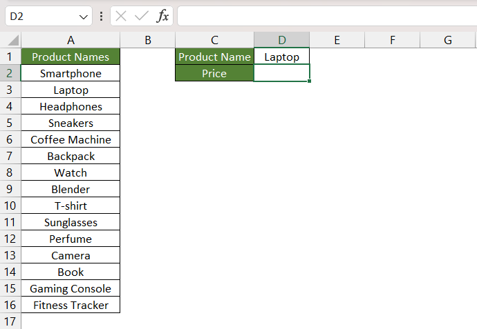
Imagine you have a Product List and seek to determine the position of a specific item within this list. In such a scenario, the MATCH function would come into play.

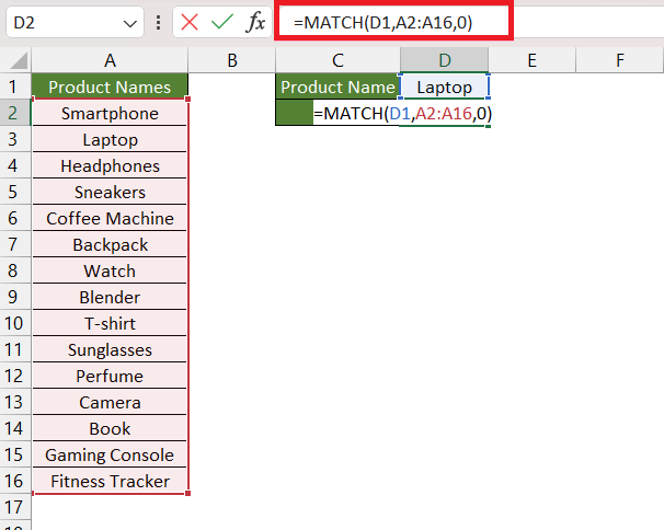
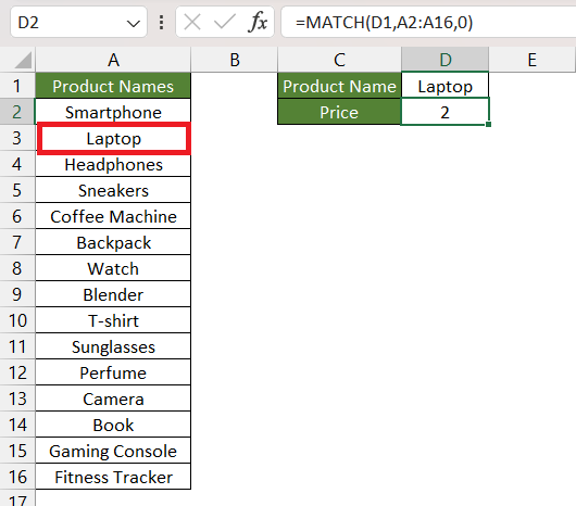
Let’s use the MATCH function to determine the position of the Laptop in the list provided.

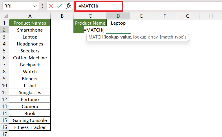
STEP 1: Enter the MATCH function.

=MATCH(

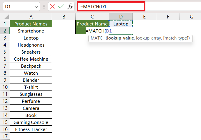
STEP 2: Enter the first argument i.e. lookup_value. Here, it is Laptop mentioned in cell D1.

=MATCH(D1, 

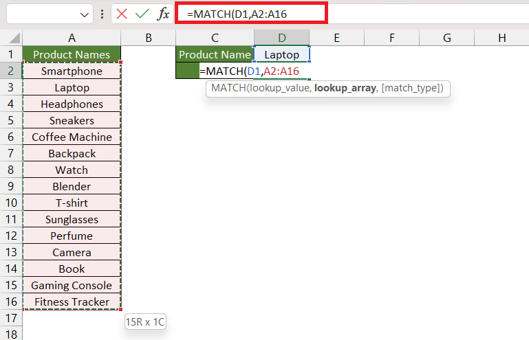
STEP 3: Enter the second argument i.e. lookup_array. Here, it is mentioned in cell A2:A16.

=MATCH(D1,A2:A16,

STEP 4: Enter the second argument i.e. match_type. Here, it is 0 for an exact match.

=MATCH(D1,A2:A16,0)

The position of the Laptop is 2 in the list.

 

Approximate Match

For an approximate match search, you must configure the match_type to either 1 (exact match or nearest smaller value) or -1 (exact match or nearest smaller value).

• If you need an exact match or nearest smaller value; you need to sort the data in ascending order.
• If you need an exact match or nearest larger value; you need to sort the data in descending order.

The approximate match is useful when you have a range of values representing sales figures and you want to find the position of the highest value that’s less than or equal to a certain target.

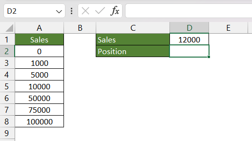
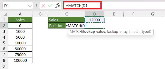
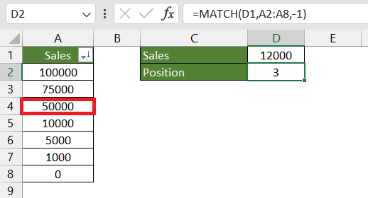
In the example shown below, there is a range of values representing sales figures and you want to find the position of the highest value that’s less than or equal to a certain target. We need to know the position of sales amount – $12,000 with the help of the Match function.

Follow the steps below to achieve the results –

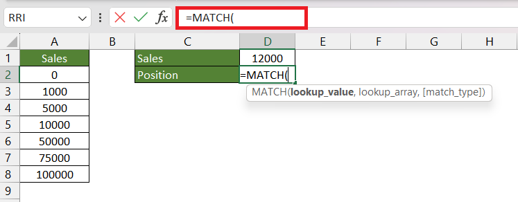
STEP 1: Enter the MATCH function.

=MATCH(

STEP 2: Enter the first argument i.e. lookup_value. Here, it is Laptop mentioned in cell D1.

=MATCH(D1, 

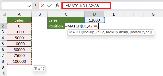
STEP 3: Enter the second argument i.e. lookup_array. Here, it is mentioned in cell A2:A16.

=MATCH(D1,A2:A8,

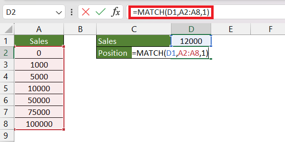
STEP 4: Enter the second argument i.e. match_type. Here, it is 1 as we need to know the position for an exact match or the next smaller.

=MATCH(D1,A2:A8,1)

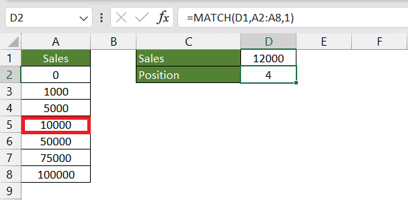
Since the next smallest value for 12,000 is 10,000; Excel has displayed the result as the position of 10000 i.e. 4.

Now, if we want to search for the next largest value, replace the third argument with -1. Here, since the next larger value is 50000, Excel has displayed the position of 50000 i.e. 3.

=MATCH(D1,A2:A8,-1)

 

Wildcard MATCH

Wildcards in Excel are special characters that you can use as placeholders to represent one or more characters in a text string. It can be used when you are unsure about the exact characters present at a specific location.

There are two main wildcards used in Excel:

1. Asterisk (*) – The asterisk wildcard represents any sequence of characters, including no characters. For example:
   • “app*” can match “apple,” “application,” “approve,” etc.
   • “*ing” can match “singing,” “running,” “writing,” etc.
2. Question Mark (?) – The question mark wildcard represents any single character. For example:
   • “h?t” can match “hat,” “hot,” “hit,” etc.
   • “?it” can match “sit”, “hit”, etc.

Let us look at an example to understand how to use wildcards in the MATCH function in Excel.

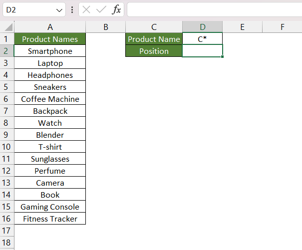
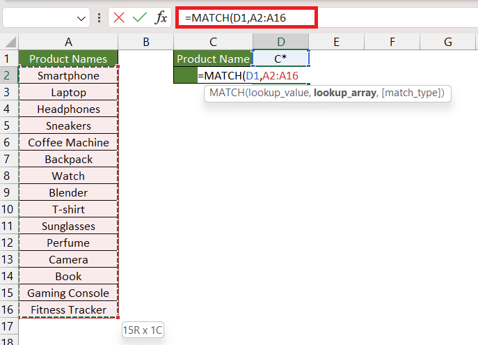
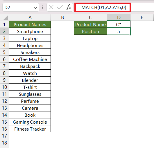
Here, we want to know the position of the product name starting with C.

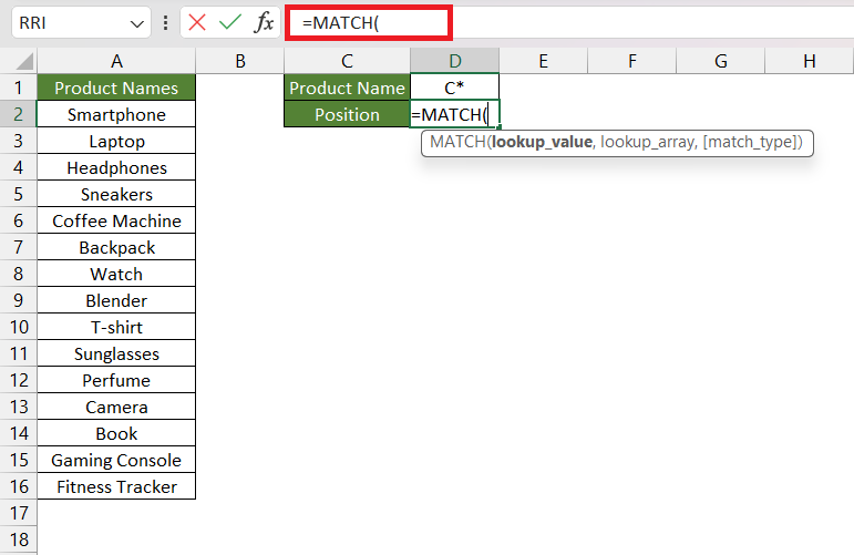
STEP 1: Enter the MATCH function.

=MATCH(

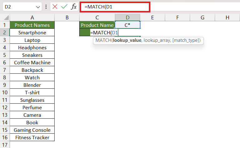
STEP 2: Enter the first argument i.e. lookup_value. Here, it is “C*” mentioned in cell D1.

=MATCH(D1, 

By incorporating asterisks behind the letter C, the function searches for any product name starting with the letter C.

STEP 3: Enter the second argument i.e. lookup_array. Here, it is mentioned in cell A2:A16.

=MATCH(D1,A2:A16,

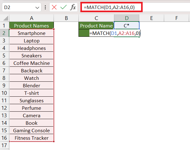
STEP 4: Enter the second argument i.e. match_type. Here, it is 0 for an exact match.

=MATCH(D1,A2:A16,0)

Here is the result!

 

Conclusion

The MATCH function in Excel is a powerful tool that allows you to search for a specified value in a range of cells and returns the relative position of that value within the range. From exact, approximate, to wildcard matches, MATCH empowers users to locate data points precisely and adapt to dynamic patterns.

Further Learning:

• INDEX and MATCH Made Simple
• Match Two Lists With The MATCH Function
• INDEX-MATCH Maximum Sales

Click here to learn all about it!