The best thing is it gives you full control over how you want your final table to look. Let us see how we can achieve this!
Exercise Workbook:
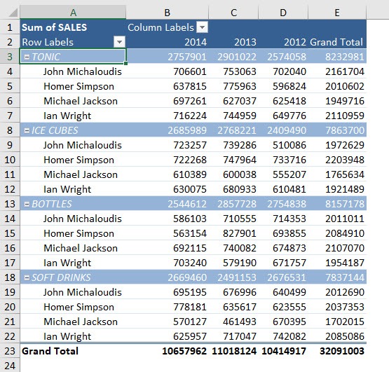
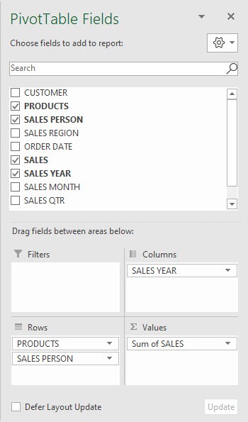
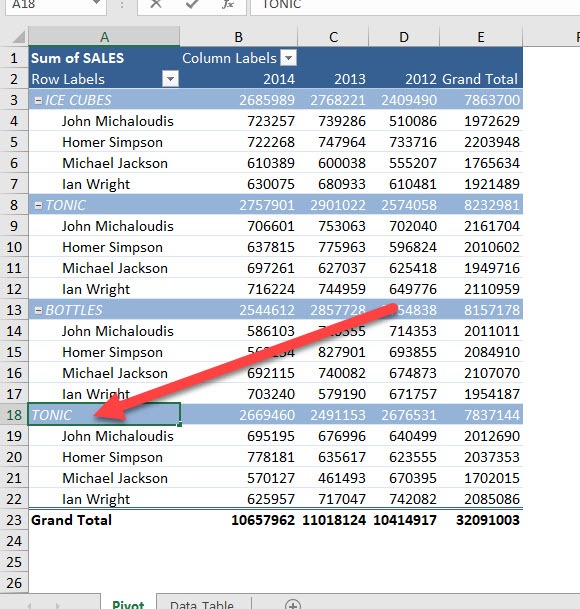
Here is how our Pivot Table is currently setup:
STEP 1: Let us work with rows first. Let’s move the TONIC row down one spot.
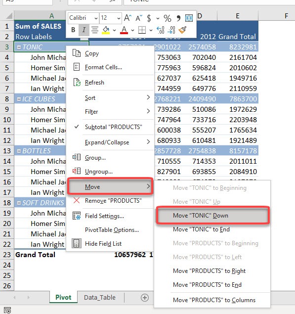
Right click on the TONIC row and go to Move > Move “TONIC” Down
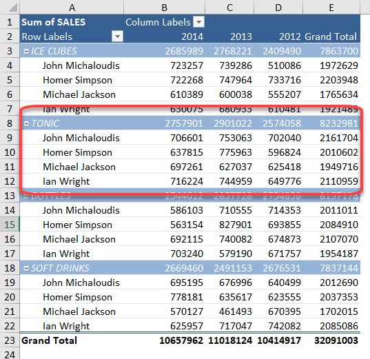
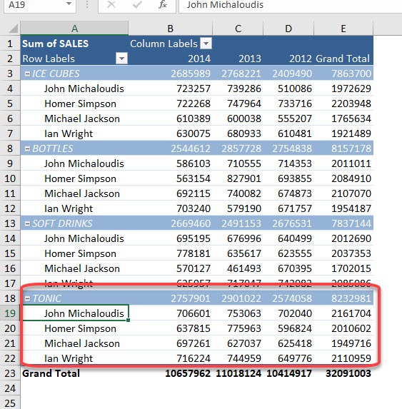
It now moved one spot below
STEP 2: You can also move it by typing the value as well!
Let us move it to the last Product row. Type in TONIC at the last Product row.
And just like that it has now moved to the bottom!
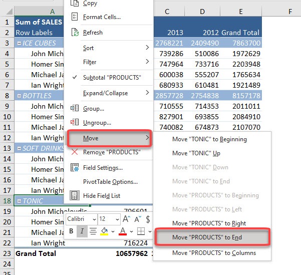
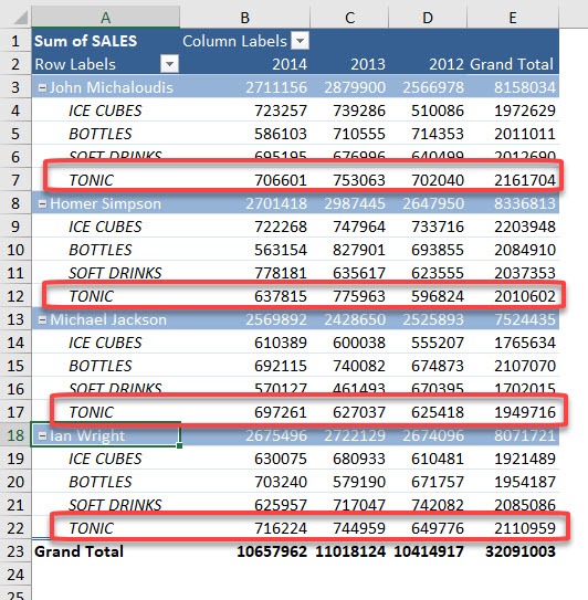
STEP 3: What if we want to update the hierarchy of our Fields? Right click on any Product row and go to Move > Move “PRODUCTS” To End
Now it’s the Salesperson that is now showing the Product Details
STEP 4: The same tips apply for the columns as well. Let us try it out!
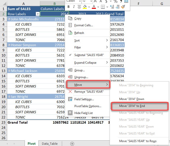
Let’s move the 2014 column to the very end.
Right click on the 2014 column and go to Move > Move “2014” to End
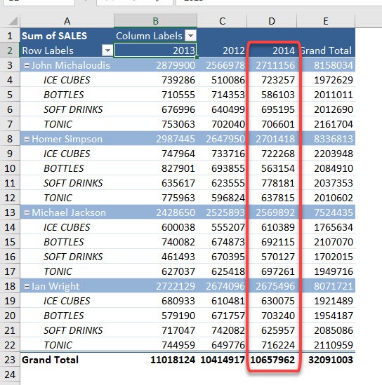
And there you have it!
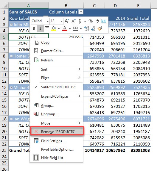
STEP 5: To remove the field. You simply right click on the field and select Remove.
In our scenario, right click on BOTTLES and select Remove “PRODUCTS”
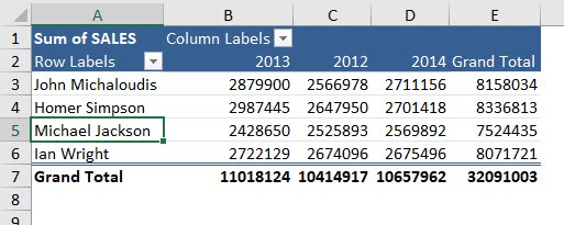
You are now left with the Salesperson field for your rows!
This is how you easily move and remove fields and items in Pivot Table. Click Here to know all about this powerful tool – Excel Pivot Tables!
Make sure to download our FREE PDF on the 333 Excel keyboard Shortcuts here:
Bryan
Bryan is a best-selling book author of the 101 Excel Series paperback books.
