We love using slicers, it just adds a level of interactivity in our reports. Did you know you can now multi-select slicer items as well?
With just a click on your slicer, you can now enable this!
This is our data that we will use for the Slicer.
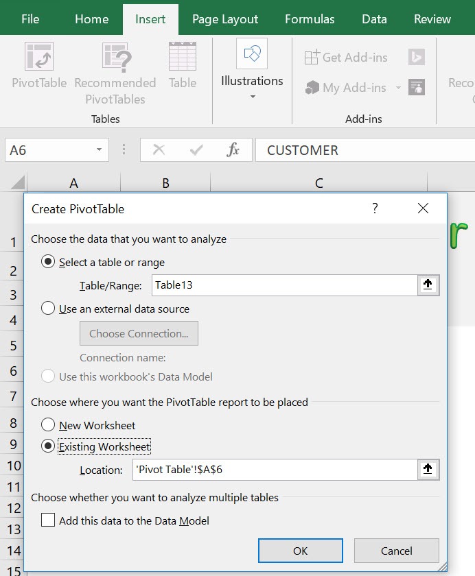
STEP 1: Insert a new Pivot table by clicking on your data and going to Insert > Pivot Table > New Worksheet or Existing Worksheet
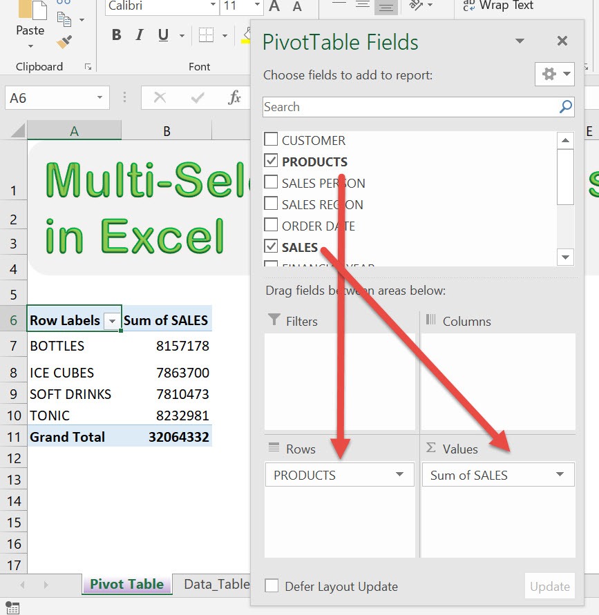
STEP 2: In the ROWS section put in the Products field. In the VALUES section put in the Sales field.
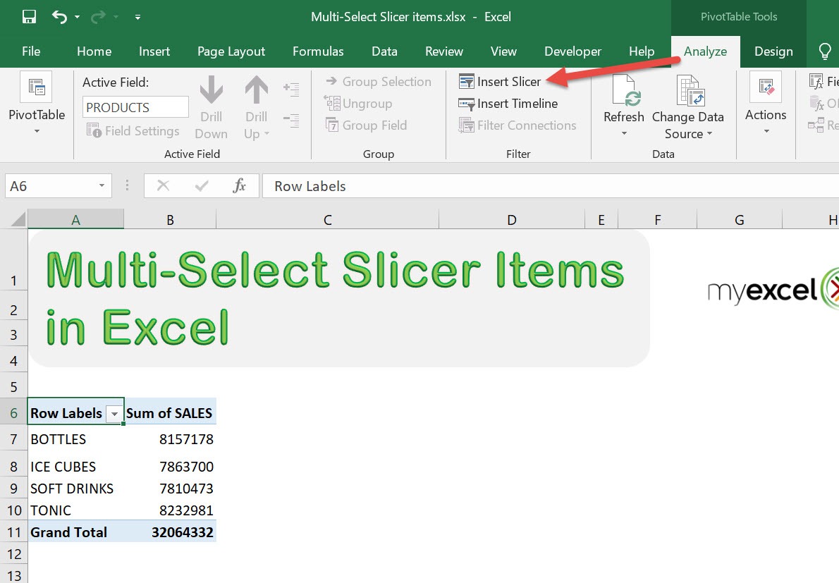
STEP 3: Let us now add our slicer! Go to PivotTable Tools> Analyze > Filter > Insert Slicer
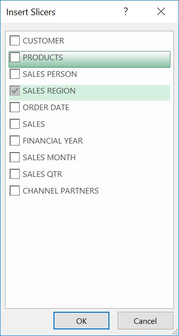
STEP 4: Make sure SALES REGION is ticked. Click OK.
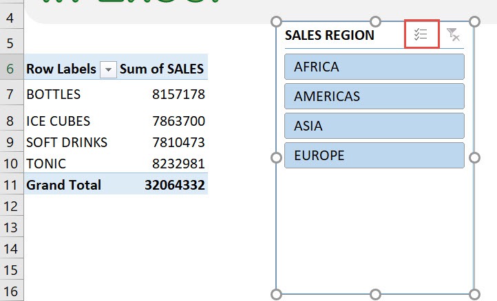
And now you have your Slicer! We just need to tick the Multi-Select button to enable this:
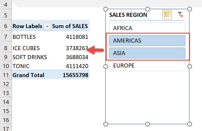
And just that, you can now multi-select slicer items! See here we have now selected Americas and Asia:
How to Multi-Select Slicer Items in Excel Pivot Tables
Helpful Resource:
Bryan
Bryan is a best-selling book author of the 101 Excel Series paperback books.


