This is your one stop shop on learning the new formulas in Excel 2019: CONCAT, IFS, MAXIFS, MINIFS, SWITCH and TEXTJOIN!
Table of Contents
Want to Master the New Formulas in Excel 2019?
*** Watch our video and step by step guide below with free downloadable Excel workbook to practice ***
CONCAT FORMULA
What does it do?
Concatenates a list together without a delimiter
Formula breakdown:
=CONCAT(text1, [text2], …)
What it means:
=CONCAT(first text to combine, [second text to combine], …)
Do you want to combine text or a range of cells together easily? The CONCAT Formula in Excel will do this for you in a flash! The CONCAT Formula was introduced in Excel 2019.
It will simply combine the text you specify together into a single text.
I explain how you can do this below:
STEP 1: We need to enter the CONCAT function in a blank cell:
=CONCAT(
STEP 2: The CONCAT arguments:
text1, …
Which cells do you want to combine together?
Select the range of cells that you want to combine together
=CONCAT(C9:E9)
Apply the same formula to the rest of the cells by dragging the lower right corner downwards.
You now have your combined text!
IFS FORMULA
What does it do?
Checks multiple conditions and returns the value of the first TRUE condition
Formula breakdown:
=IFS(logical_test1, value_if_true1, [logical_test2, value_if_true2], …)
What it means:
=IFS(first condition to check, value to return, [succeeding conditions to check], …)
If you have multiple logical conditions to check, instead of creating Nested IF Formulas, we can use Excel’s IFS Formula! It allows us to specify multiple conditions to check, then the IFS Formula will look for the first condition that gets satisfied!
Let us try it out on a simple tax table, then we will create an IFS Formula that will simulate the exact same logic of the table!
I explain how you can do this below:
STEP 1: We need to enter the IFS function in a blank cell:
=IFS(
STEP 2: The IFS arguments:
logical_test1, value_if_true1
What is the first condition and value to return if the condition is met?
Let us start from the minimum value of the tax table. If the income is less than $8456, then the tax rate is 13%
=IFS(G8<8456, 13%,
logical_test2, value_if_true2
What is the second condition and value to return if the condition is met?
Going to the second row, if the income is less than $15874, then the tax rate is 18%
=IFS(G8<8456, 13%, G8<15874, 18%,
logical_test3, value_if_true3
What is the third condition and value to return if the condition is met?
Going to the last row, if the income is greater than or equal to $15874, then the tax rate is 22%
=IFS(G8<8456, 13%, G8<15874, 18%, G8>=15874, 22%)
You now have your correct tax rate!
MAXIFS FORMULA
What does it do?
Gets the max value based on the cells that matches the criteria
Formula breakdown:
=MAXIFS(max_range, criteria_range1, criteria1, …)
What it means:
=MAXIFS(cells that contains the values, first set of cells to base the filtering on, filtering condition of first set of cells, …)
If you need to get the max value while doing filtering at the same time, the MAXIFS Formula will do this for you in Excel! This was introduced in Excel 2019.
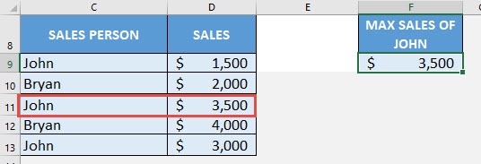
You need to specify on which ones you want to get the MAX value, then specify one or more conditions used for filtering. In our example, we want to get the maximum sales of John!
I explain how you can do this below:
STEP 1: We need to enter the MAXIFS function in a blank cell:
=MAXIFS(
STEP 2: The MAXIFS arguments:
max_range
What is the range that contains the values to get the max value?
Select the cells containing the sales numbers that you want to get the maximum value from:
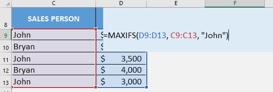
=MAXIFS(D9:D13,
criteria_range1
What is the range that contains the values for filtering?
Select the cells containing the sales person names:
=MAXIFS(D9:D13, C9:C13,
criteria1
What is the your filtering criteria?
Since we want to filter to the sales numbers of John, type in John:
=MAXIFS(D9:D13, C9:C13, “John”)
You now have John’s highest sales number!
MINIFS FORMULA
What does it do?
Gets the minimum value based on the cells that matches the criteria
Formula breakdown:
=MINIFS(min_range, criteria_range1, criteria1, …)
What it means:
=MINIFS(cells that contains the values, first set of cells to base the filtering on, filtering condition of first set of cells, …)
If you need to get the minimum value while doing filtering at the same time, the MINIFS Formula will do this for you in Excel! This was introduced in Excel 2019.
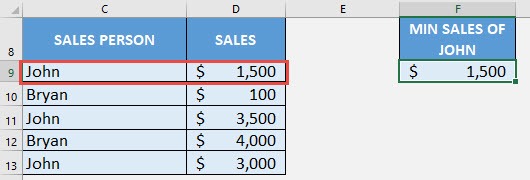
You need to specify on which ones you want to get the MIN value, then specify one or more conditions used for filtering. In our example, we want to get the minimum sales of John!
I explain how you can do this below:
STEP 1: We need to enter the MINIFS function in a blank cell:
=MINIFS(
STEP 2: The MINIFS arguments:
min_range
What is the range that contains the values to get the min value?
Select the cells containing the sales numbers that you want to get the minimum value from:
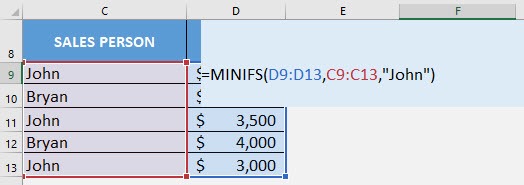
=MINIFS(D9:D13,
criteria_range1
What is the range that contains the values for filtering?
Select the cells containing the sales person names:
=MINIFS(D9:D13, C9:C13,
criteria1
What is the your filtering criteria?
Since we want to filter to the sales numbers of John, type in John:
=MINIFS(D9:D13, C9:C13, “John”)
You now have John’s lowest sales number!
SWITCH FORMULA
What does it do?
Matches multiple values and returns the first value that has a match
Formula breakdown:
=SWITCH(expression, value1, result1, [value2 / default, result2], …)
What it means:
=SWITCH(value to check, value to match against, result to return, [succeeding values to match or the default value if nothing gets matched], …)
If you have multiple values to check, we can use Excel’s SWITCH Formula! It allows us to specify multiple values to check, then the SWITCH Formula will look for the first value that gets matched!
Let us try it out on a simple ratings table (e.g. 1 = Bad, 2 = Average, 3 = Great), then we will create a SWITCH Formula that will simulate the exact same logic of the table!
I explain how you can do this below:
STEP 1: We need to enter the SWITCH function in a blank cell:
=SWITCH(
STEP 2: The SWITCH arguments:
expression
What is the value to check?
Select the cell containing the rating that you want to translate to the correct description
=SWITCH(G8,
value1, result1
What is the first lookup value and value to return if it is matched?
Let us start from the first value of the rating table. If the value is 1, then the description is “Bad”
=SWITCH(G8, 1, “Bad”
value2, result2
What is the second lookup value and value to return if it is matched?
Let us start from the second value of the rating table. If the value is 2, then the description is “Average”
=SWITCH(G8, 1, “Bad”, 2, “Average”,
value3, result3
What is the third lookup value and value to return if it is matched?
Let us start from the third value of the rating table. If the value is 3, then the description is “Great”
=SWITCH(G8, 1, “Bad”, 2, “Average”, 3, “Great”,
default
What is the default value to return if nothing gets matched?
We want to show the value “Unknown”, if an unknown rating is specified.
=SWITCH(G8, 1, “Bad”, 2, “Average”, 3, “Great”, “Unknown”)
You now have your correct rating description!
Let us try an unknown rating (40) and see the resulting description:
TEXTJOIN FORMULA
What does it do?
Concatenates a list with a specified delimiter
Formula breakdown:
=TEXTJOIN(delimiter, ignore_empty, text1, …)
What it means:
=TEXTJOIN(the delimiter, ignore empty cells in combining text, first text/range to combine, …)
Do you want to combine text or a range of cells together easily? The TEXTJOIN Formula in Excel will do this for you in a flash! The TEXTJOIN Formula was introduced in Excel 2019.
It can even let you specify a delimiter to use to combine the text together and ignore empty cells for you!
I explain how you can do this below:
STEP 1: We need to enter the TEXTJOIN function in a blank cell:
=TEXTJOIN(
STEP 2: The TEXTJOIN arguments:
delimiter
What is the delimiter to use in combining the text?
We want to have the text combined together and separated by a comma:
=TEXTJOIN(“,”,
ignore_empty
Do you want to ignore the empty cells?
Let us set this to TRUE to ignore the empty cells when combining them together:
=TEXTJOIN(“,”, TRUE,
text1, …
Which cells do you want to combine together?
Select the range of cells that you want to combine together
=TEXTJOIN(“,”, TRUE, C9:E9)
Apply the same formula to the rest of the cells by dragging the lower right corner downwards.
You now have your combined text!
Bryan
Bryan is a best-selling book author of the 101 Excel Series paperback books.


