This is your one stop shop on learning the new Excel formulas in Office 365: FILTER, RANDARRAY, SEQUENCE, SORT, SORTBY and UNIQUE!
Table of Contents
Want to Master the New Excel Formulas in Office 365?
*** Watch our video and step by step guide below with free downloadable Excel workbook to practice ***
What does it do?
Filters a table array based on the filtering condition given
Formula breakdown:
=FILTER(array, include, [if_empty])
What it means:
=FILTER(data to be filtered, the filtering condition, [value to display if nothing gets matched])
Did you know that you can now filter your table data with an Excel Formula? Yes you can! It is definitely possible now with Excel’s FILTER Formula. It is a new formula introduced in Office 365 released in 2018!
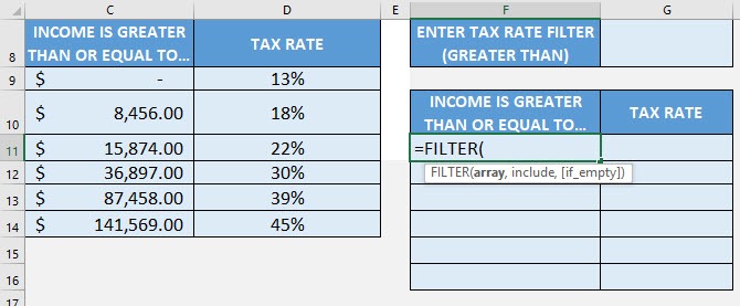
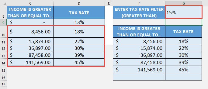
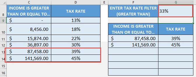
We have a tax table that we want to dynamically filter with a given rate.
I explain how you can do this below:
STEP 1: We need to enter the FILTER function in a blank cell:
=FILTER(
STEP 2: The FILTER arguments:
array
What is the data to be filtered?
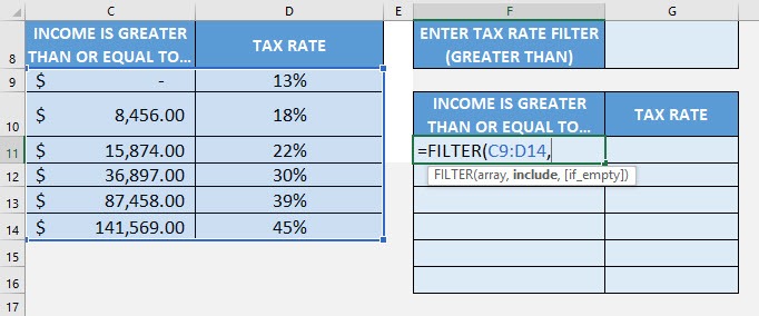
Select the cells containing the tax data, do not include the headers:
=FILTER(C9:D14,
include
What is your filtering condition?
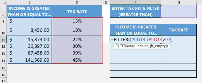
We want to filter the tax rate that is greater than the specified rate. Type in the condition as the tax rate column > the specific tax rate.
=FILTER(C9:D14, D9:D14>G8
[if_empty]
What is the value to display in case nothing gets matched?
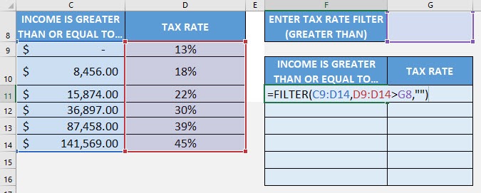
Just place an empty string to be displayed if nothing gets matched.
=FILTER(C9:D14, D9:D14>G8, “”)
Try it out now with different values and see it get filtered magically!
RANDARRAY FORMULA
What does it do?
Creates an array of random numbers
Formula breakdown:
=RANDARRAY([rows], [columns])
What it means:
=RANDARRAY(number of rows, number of columns)
Did you know that you can now generate random numbers in an array? Yes you can! It is definitely possible now with Excel’s RANDARRAY Formula. It is a new formula introduced in Office 365 released in 2018!
It returns random values between 0 and 1 by default. I explain how you can do this below:
STEP 1: We need to enter the RANDARRAY function in a blank cell:
=RANDARRAY(
STEP 2: The RANDARRAY arguments:
[rows]
How many rows to fill random values with?
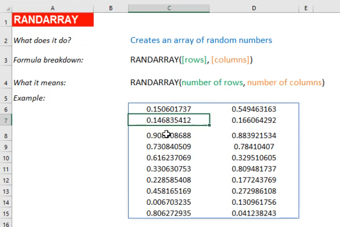
Let us go for 10 rows.
=RANDARRAY(10,
[columns]
How many columns to fill random values with?
Let us go for 2 columns.
=RANDARRAY(10, 2)
Now we have our 10 x 2 area filled with random values between 0 and 1!
SEQUENCE FORMULA
What does it do?
Creates an array of sequential numbers
Formula breakdown:
=SEQUENCE(rows, [columns], [start], [step])
What it means:
=SEQUENCE(number of rows, [number of columns], [starting number], [increment per number])
Did you know that you can now generate a series of numbers with an Excel Formula? Yes you can! It is definitely possible now with Excel’s SEQUENCE Formula. It is a new formula introduced in Office 365 released in 2018!
I explain how you can do this below:
STEP 1: We need to enter the SEQUENCE function in a blank cell:
=SEQUENCE(
STEP 2: The SEQUENCE arguments:
rows
How many rows to fill with values?
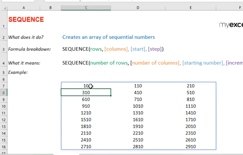
Let us go for 10 rows.
=SEQUENCE(10,
[columns]
How many columns to fill with values?
Let us go for 3 columns.
=SEQUENCE(10, 3,
[start]
Which number do you want the sequence of numbers to start?
Let us have it start at the number 10.
=SEQUENCE(10, 3, 10,
[step]
Which increment for each number in the sequence?
Let us increment it by 100. So that numbers should look like: 10, 110, 210, 310, and so on…
=SEQUENCE(10, 3, 10, 100)
Try it out now and see that your sequence of numbers is generated magically!
SORT FORMULA
What does it do?
Sorts a table based on a column and order specified
Formula breakdown:
=SORT(array, [sort_index], [sort_order])
What it means:
=SORT(data to be sorted, [which column to be used for sorting], [ascending or descending order])
Did you know that you can now sort your table data with an Excel Formula? Yes you can! It is definitely possible now with Excel’s SORT Formula. It is a new formula introduced in Office 365 released in 2018!
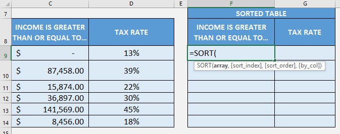
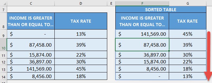
We have a tax table that we want to sort by the tax rate in a descending order.
I explain how you can do this below:
STEP 1: We need to enter the SORT function in a blank cell:
=SORT(
STEP 2: The SORT arguments:
array
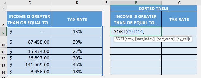
What is the data to be sorted?
Select the cells containing the tax data, do not include the headers:
=SORT(C9:D14,
[sort_index]
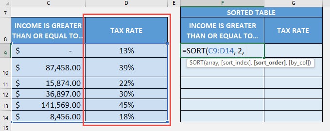
What is the column to be used for sorting?
We specify the column number here. Since the tax rate column is the second column, place in 2.
=SORT(C9:D14, 2,
[sort_order]
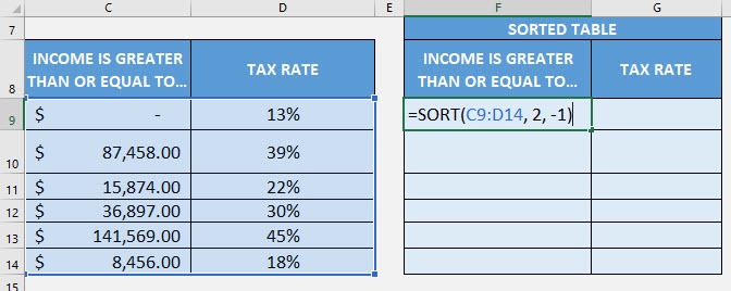
What is the sort order? 1 for Ascending, -1 for Descending order.
Since we want descending order, place in -1.
=SORT(C9:D14, 2, -1)
Now it gets sorted magically!
SORTBY FORMULA
What does it do?
Sorts a table based on the column(s) specified
Formula breakdown:
=SORTBY(array, by_array1, sort_order1, [by_array2, sort_order2], …)
What it means:
=SORTBY(data to be sorted, by which column to sort first, [by which column to sort afterwards], …)
Did you know that you can now sort your table data with an Excel Formula? Yes you can! It is definitely possible now with Excel’s SORTBY Formula. It also allows you to sort by multiple columns as well. It is a new formula introduced in Office 365 released in 2018!
We have a person list that we want to sort by Gender (ascending order) and then by Age (ascending order).
Do take note that in specifying the sorting order, 1 represents ascending order, -1 represents descending order.
I explain how you can do this below:
STEP 1: We need to enter the SORTBY function in a blank cell:
=SORTBY(
STEP 2: The SORTBY arguments:
array
What is the data to be sorted?
Select the cells containing the person data, do not include the headers:
=SORTBY(B9:D14,
by_array1, sort_order1
Which column will be used to sort first?
Select the cells containing the gender column, then type in 1 for it to be ascending order.
=SORTBY(B9:D14, B9:B14, 1,
by_array2, sort_order2
Which column will be used to sort next?
Select the cells containing the age column, then type in 1 for it to be ascending order.
=SORTBY(B9:D14, B9:B14, 1, D9:D14, 1)
Now it gets sorted magically!
UNIQUE FORMULA
What does it do?
Gets the unique values of a list
Formula breakdown:
=UNIQUE(array)
What it means:
=UNIQUE(data to have duplicates removed)
Want to remove duplicate values from your list? It is definitely possible now with Excel’s UNIQUE Formula. It is a new formula introduced in Office 365 released in 2018!
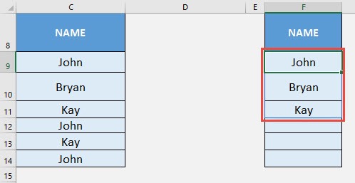
We have a list of names and we want to remove the duplicates from it. The UNIQUE Formula will make this very quick to do!
I explain how you can do this below:
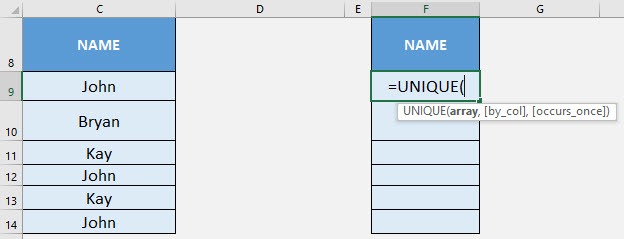
STEP 1: We need to enter the UNIQUE function in a blank cell:
=UNIQUE(
STEP 2: The UNIQUE arguments:
array
What is the data to be cleared of duplicate values?
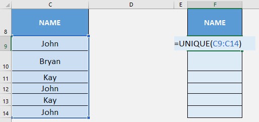
Select the cells containing the names, do not include the headers:
=UNIQUE(C9:C14)
Now the duplicate names are all gone!
Bryan
Bryan is a best-selling book author of the 101 Excel Series paperback books.

