In the world of Microsoft Excel, mastering percentage formatting is a crucial skill for anyone involved in data analysis. Whether you’re comparing sales figures, demographic statistics, or financial data, percentages offer a streamlined method for making meaningful comparisons across different scales. This guide will walk you through the process of adding percentage signs to your Excel sheets effortlessly.
Key Takeaways:
- Understand how percentages serve as the cornerstone of data analysis, providing a universal language for comparison and interpretation across diverse datasets.
- Learn the easy steps to apply percentage formatting in Excel, transforming raw numbers into easily understandable insights with just a few clicks.
- Discover shortcuts and techniques to format numbers as percentages as you type, enhancing your efficiency and workflow within Excel.
- Tailor your percentage formatting to meet specific analytical needs by adjusting decimal places and employing custom formats, ensuring clarity and accuracy in your data presentations.
Table of Contents
Introducing Percentage Formatting in Excel
Understanding the Role of Percentages in Data Analysis
Percentages are the bread and butter of data analysis, offering a harmonious way to compare figures from different-sized categories. They level the playing field, allowing you to see proportions and make relative comparisons across your data.
Imagine you’re juggling datasets from various departments or demographic groups; percentages are your ally, transforming raw numbers into relatable insights that are easier to digest and act upon.
The Basics of Adding Percentage Signs in Excel
Adding a percentage sign in Excel is as simple as pie, turning a decimal or fraction into a clear percentage with just a few clicks. When you type numbers in Excel and visualize them as portions of 100, that’s when you should call on the almighty percentage sign to make sense of them.
To get the ball rolling, you’ll typically highlight your desired cells and tap on the percentage symbol right under the ‘Home’ tab. Or, if you prefer a different route, right-click the cell, choose ‘Format Cells,’ select ‘Percentage,’ and voila! Your simple decimals now have their “%” sidekick, making your data snappier and more informative.
Step-by-Step Guide to Format Numbers as Percentages
Applying the Percentage Format to Existing Values
Ever tried adding a percentage format to numbers that already exist in your spreadsheet, only to find them ballooning to unexpected values? You’re not alone. Excel is a bit overzealous and likes to multiply your numbers by 100 when you slap on a percentage format. To tackle this head-on, just roll up your sleeves and divide those numbers by 100 first, or enter them in decimals from the get-go.
For a smooth transition, use a simple formula.
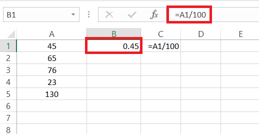
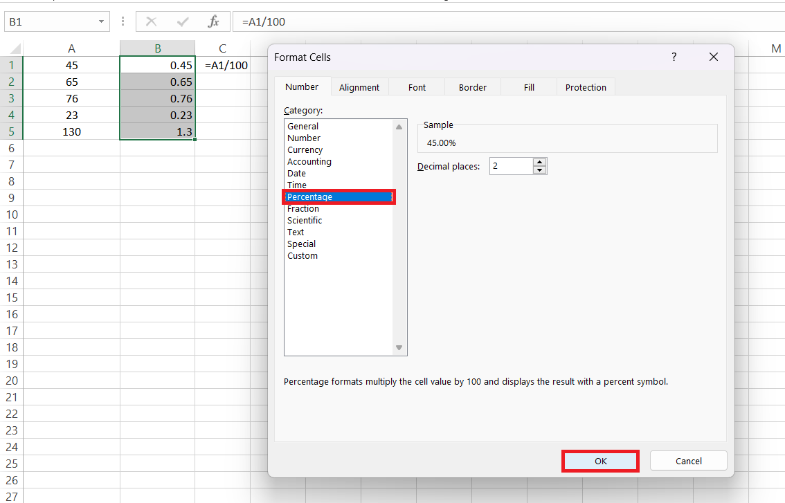
STEP 1: Imagine having your starting number in cell A1; in the next cell, just type =A1/100, then copy-paste this formula down the column.
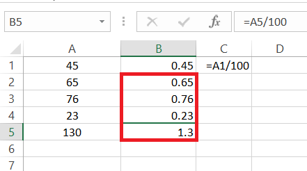
STEP 2: Now drag and drop the formula from cell B2 until B5.
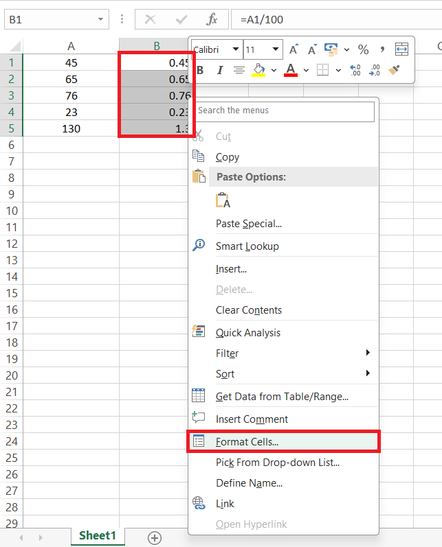
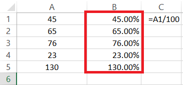
STEP 3: Once you’ve done that, you can format this new column with the percentage style, by selecting the cells then clicking right > choose “Format Cells”.
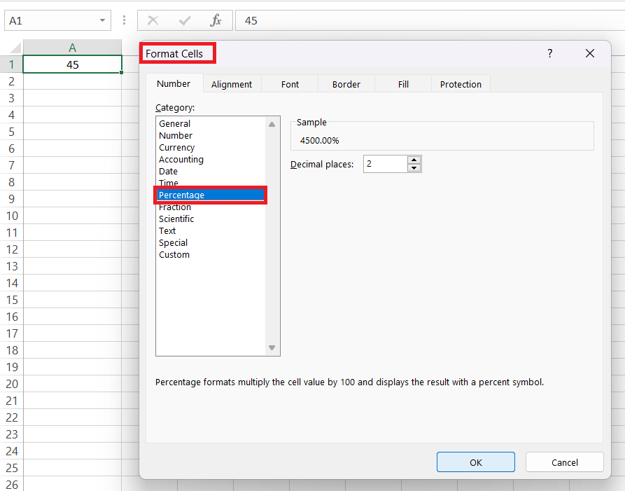
STEP 4: Select “Percentage” from the Format Cells dialog box. Lastly, hit “OK”.
Boom—a perfect conversion to percentages.
Additionally, once your numbers look how you want them to, you can convert these formulas to static values by copying and pasting them as ‘Values’. This little trick helps you prevent any accidental changes if you later change the values in the original A1 cell.
Displaying Numbers as Percentages as You Type
Now, if you’re someone who prefers to dress numbers in percentage garb as you type, step right up—it’s easy with Excel’s flexible formatting.
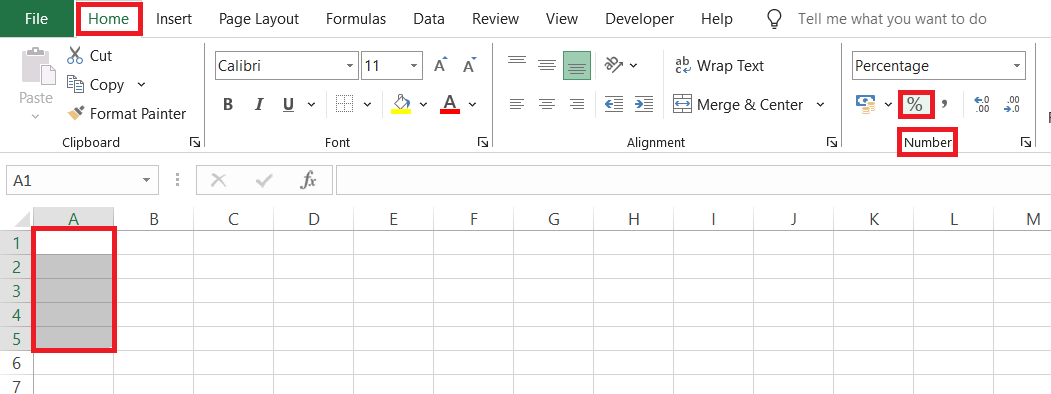
STEP 1: Just select your battlefield (the cells where you want to enter percentages), go to the ‘Home’ tab, and pick ‘Percentage’ from the ‘Number’ group. This preps your cells, so they’re ready to interpret anything you type as a percentage.
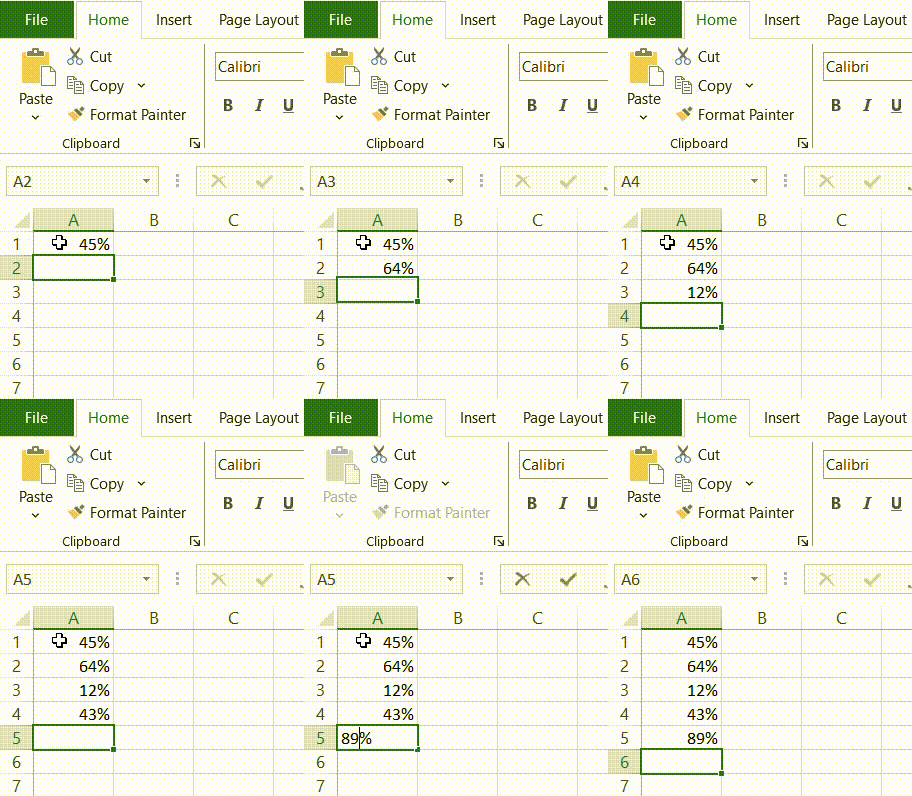
RESULT:
If you’re all about efficiency and key shortcuts rock your world, don’t forget to press “Ctrl+Shift+%” after selecting your cells. Type your numbers, punch in Enter, and watch as Excel automatically endows them with the coveted percentage symbol, like a math magician impressing the crowd.
Customizing Your Percentage Formatting
Adjusting Decimal Places for More Precise Percentages
Adjusting the decimal places is key to refine your percentages down to the exact detail. This precision lets you present data with the clarity and specificity your analysis calls for. Fiddle with the decimal points by opening the Format Cells dialog box — it’s Ctrl + 1 for the shortcut aficionados — and navigating to the ‘Percentage’ option. There, you control the decimal realm, increasing or decreasing the digits after the dot to your heart’s content.
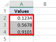
Example Dataset: Suppose you have a column of numbers representing sales percentages:
STEP 1: Highlight the cells containing your percentages.
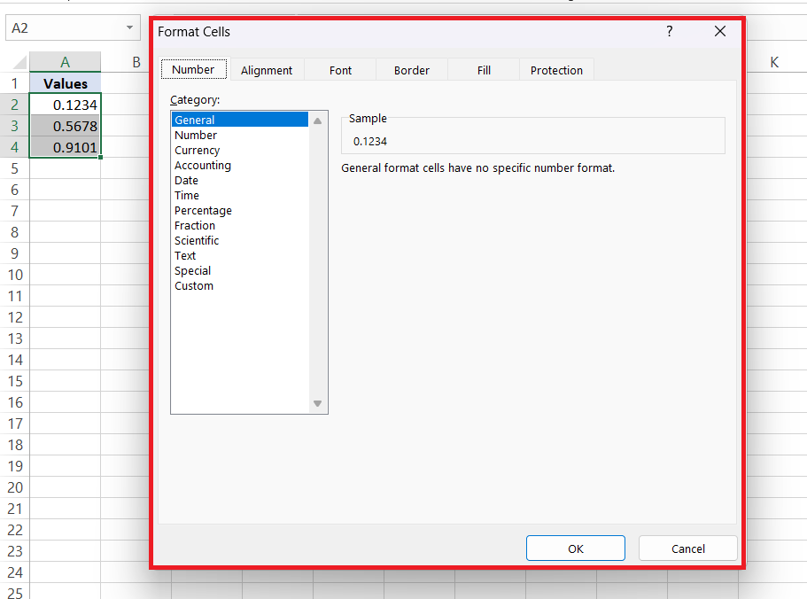
STEP 2: Press Ctrl + 1 or right-click and select “Format Cells.”
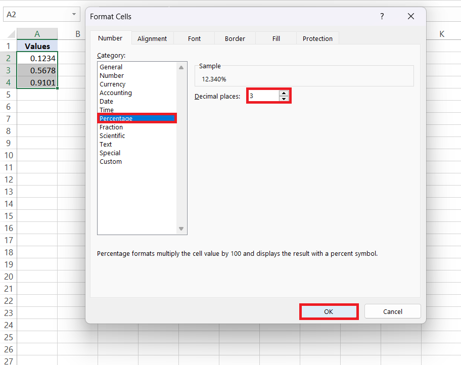
STEP 3: In the Format Cells dialog box, go to the “Number” tab and select “Percentage.” Adjust the decimal places as needed, such as here selecting “3” for two decimal places.
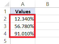
By following these steps, you can refine the precision of your percentages in Excel to meet your analytical requirements.
This small tweak can mean the difference between a rounded approximate and an exact value, crucial when dealing with sensitive financial data or when aiming for precision in scientific calculations. So whether you’re happy with a clean, whole number or need the rigor of two decimal places, Excel bends to your will with just a few clicks.
FAQ: Mastering Percentages in Excel
How do I add a sign in front of a percentage in Excel?
To add a sign (+/-) in front of a percentage in Excel, create a custom number format. First, select the cells with percentages, then press Ctrl + 1 to open the ‘Format Cells’ dialog. Go to ‘Custom’, and in the Type field, input +0.00%; -0.00%; 0.00%. This format adds a plus for positive, a minus for negative, and displays zero values with a percentage sign.
What is the shortcut for percentage in Excel?
The shortcut to apply percentage formatting in Excel is Ctrl+Shift+%. Select the cells you want to format and press these keys together, and Excel will instantly format your numbers as percentages. It’s a quick and handy way to switch to percentage view without the mouse!
How do I add a percentage symbol without changing the number value?
To add a percentage symbol without changing the number value in Excel, you’ll need a custom format. Select your numbers, press Ctrl + 1 to open the ‘Format Cells’ dialog, select ‘Custom’, and type 0"%" in the Type box. This way, you simply append the percentage symbol to your numbers without multiplying by 100, keeping the value intact.
Can I apply a percentage format to multiple cells at once?
Absolutely, applying a percentage format to multiple cells at once in Excel is a breeze! Just select the range of cells you aim to format — you can click and drag or use Shift with arrow keys for selection. Once highlighted, hit Ctrl+Shift+% or go to the ‘Home’ tab and choose the ‘Percent Style’ button. Your selected cells will now reflect the percentage format, all in one go.
How do I remove the percentage symbol in excel without changing values?
To remove the percentage symbol in Excel without altering the actual values, employ the custom number format. Select the cells, then hit Ctrl + 1 to fire up the ‘Format Cells’ dialog. Under ‘Custom’, input 0, and this will strip away the percentage symbols while preserving the original values as they are.
John Michaloudis is a former accountant and finance analyst at General Electric, a Microsoft MVP since 2020, an Amazon #1 bestselling author of 4 Microsoft Excel books and teacher of Microsoft Excel & Office over at his flagship Academy Online Course.
