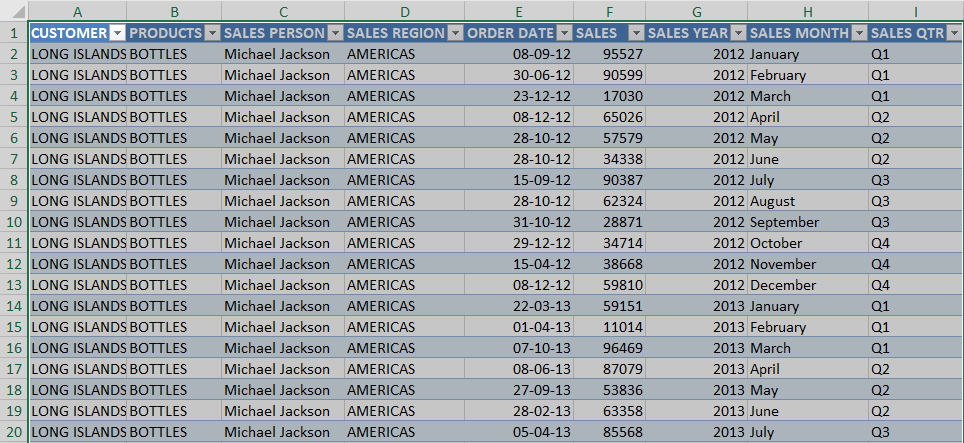
I’m going to explain to you the concept of the Pivot Cache. Join me in understanding this concept with some quick illustrative examples below!
Exercise Workbook:
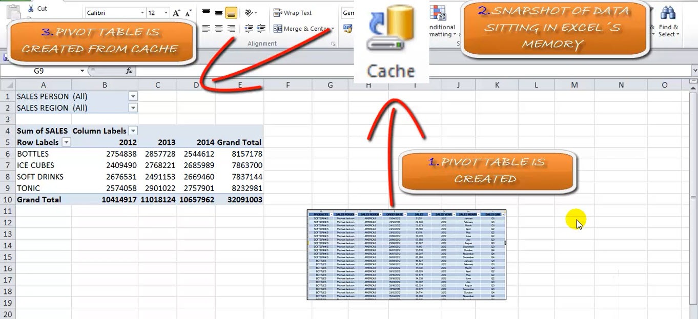
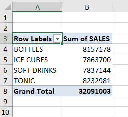
STEP 1: Why is there a need to refresh the Pivot Table? Let us look at this sequence of events below:
- You invoke the creation of the Pivot Table
- Then a snapshot of that data in that point in time is stored in the Cache
- The Cache content is the basis of how the Pivot Table is created
You do not see the Pivot Cache as this runs in the background.
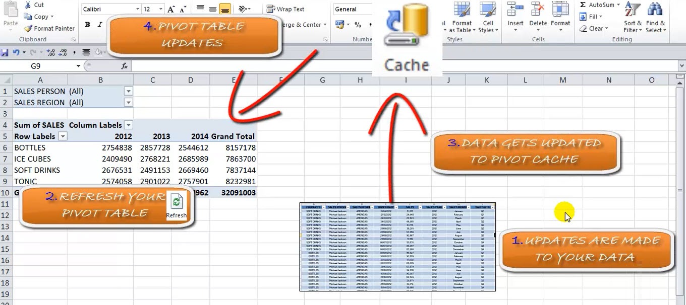
STEP 2: Now what happens when you update the source data?
- Your source data is updated
- You invoke the refreshing of the Pivot Table
- Then a snapshot of that data in that point in time is stored in the Cache
- The Pivot Table is updated based on the Cache
When you create Pivot Table in Excel, a Pivot Cache is created automatically. It is a replica of the original source data but it is not visible to us. When you make changes to the Pivot Table, it uses Pivot Cache and not the original source data.
Even though this makes Excel very responsive and quick to change, it increases the file size to almost double.
When you create multiple Pivot Tables using the same source data in a workbook, Excel creates a single Pivot Cache and re-uses it for all Pivot Tables.
The advantage of sharing a Pivot cache is that it prevents duplication but it creates several disadvantages as well:
- When you refresh one Pivot Table, all other Pivot Tables get refreshed.
- When you group one field in Pivot Table, it gets grouped in other Pivot Tables.
- When you insert a calculated field in Pivot Table, it appears on all other Pivot Tables.
If these disadvantages create a hindrance for you, you can simply create multiple Pivot caches for multiple Pivot Tables. To do so, follow the steps below:
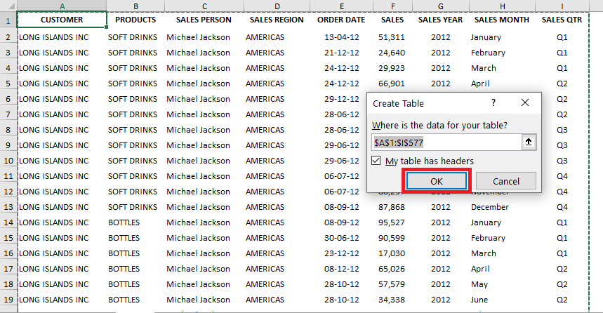
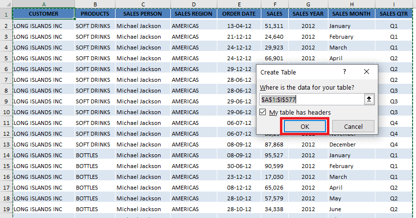
STEP 1: Click anywhere on the data source and press Ctrl + T to create a table. Click OK.
STEP 2: Go to the Table Design tab, you will see the Table Name box displaying the name (Table1) assigned to the table.
STEP 3: Select Summarize with PivotTable.
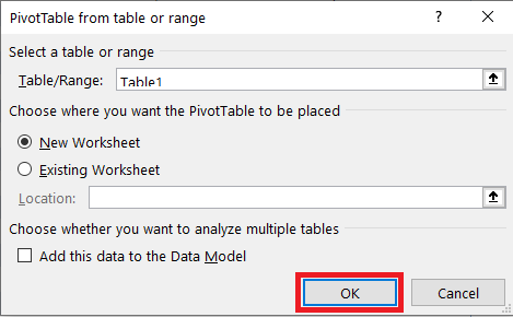
STEP 4: In the PivotTable dialog box, click OK.
Pivot Table and its cache will be created. Before you create another PivotTable, you need to covert the table back to range.
STEP 5: Go to Table Design Tab > Convert to Range.
STEP 6: Again convert the range back to a table.
Excel will assign a different name to the table – Table2.
Now you can create another Pivot Table using the data from Table2.
Since the tables have different names, Excel will create separate caches for them!
Count the Pivot Cache in Workbook
How to do how many pivot caches are present in your workbook? Excel can count them for you using a simple VBA code.
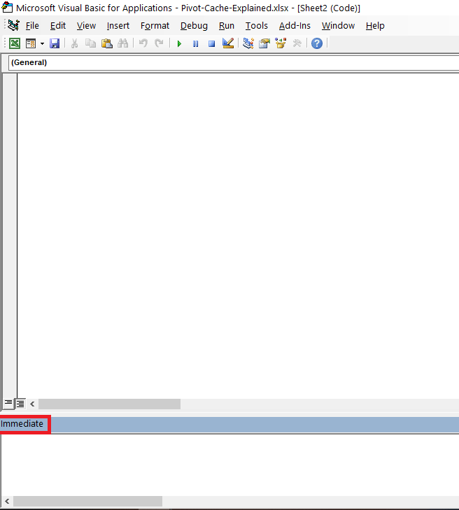
STEP 1: Press Alt + F11 to open the Visual Basic window.
STEP 2: Press Ctrl + G to open the Immediate window.
STEP 3: Enter the following code:
?ActiveWorkbook.PivotCaches.Count
STEP 4: Press Enter.
The result will be displayed below the code!
The only issue that you face while using Pivot cache is that it doubles the size of the Excel file. This problem can easily be solved by deleting the original source data. This will reduce the file size significantly!
The Pivot Table will remain intact and you can easily use it.
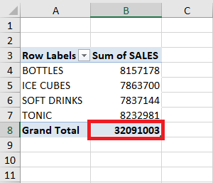
If you want to get the source data back, double click on the grand total value in the unfiltered Pivot Table.
This will paste the original source data into a new worksheet for you.
Make sure to download our FREE PDF on the 101 Best Excel Tips & Tricks:
Bryan
Bryan is a best-selling book author of the 101 Excel Series paperback books.
