There are two buttons available for customizing and formatting the Pivot Charts in Excel:
- Design Tab – It can be used to change the chart type, chart style, select data, add chart elements, etc.
- Format Tab – It can be used to change chart size, insert shapes, change shape style, etc.
Once you click on the Pivot Chart, you will have these options. Let us go over the Design and Format settings.
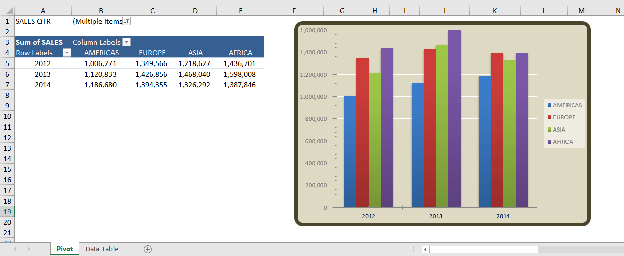
This is our current Pivot Chart that we will be using to try out the different Pivot Chart settings.
Don’t forget to download the Exercise Workbook below and follow along with us!
Design Tab
The Design tab has the following settings:
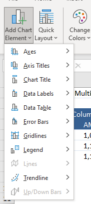
- Add Chart Element – If you want to add/remove additional elements like Axes, Data Labels, Gridlines, Legends, etc. to be displayed in your Pivot Chart, you have these settings:
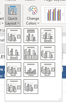
- Quick Layout – This is a handy way to have different types of presentation options. Go over them one by one to determine which will be the most appropriate way to visualize your data.
- Chart Styles – You can have fun here with the colors on how your chart will be displayed and match them with your company’s theme colors.
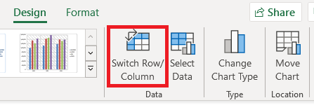
- Switch Row/Column – You can use this option to change the way data is plotted in PivotCharts. You can swap the data over the axis with this quickly and revert back when needed.
- Select Data – You can change the data source of your Pivot Chart using this option.
- Change Chart Type – There are a lot of different chart types that you can change quickly.
- Move Chart – If you need to place the Pivot Chart in a different location, you can easily use this option.
Format Tab
The Format tab has the following settings:
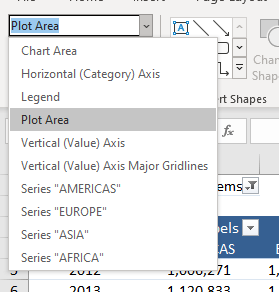
- Current Selection – You select the specific element of your Pivot Chart on the one you want to modify visually.
- Insert Shapes – You can add additional shapes that will help present your data better on top of your Pivot Chart such as arrows and boxes.
- Shape Styles – You can change the color fill, outline, or even add 3d effects to how it is displayed.
- WordArt Styles – You can change how text is formatted here with preset styles available.
- Arrange – You can change the display order, set alignment, or even rotate the selected element.
- Size – You can change the length and width here.
So, you can use the command buttons present in the Design and Format tab available for PivotCharts to easily customize and format your chart as per your requirement!
Make sure to download our FREE PDF on the 333 Excel keyboard Shortcuts here:
Bryan
Bryan is a best-selling book author of the 101 Excel Series paperback books.

