Table of Contents
Want to know How to Conditionally Format Blank Cells in Excel Pivot Tables?
*** Watch our video and step by step guide below with free downloadable Excel workbook to practice ***
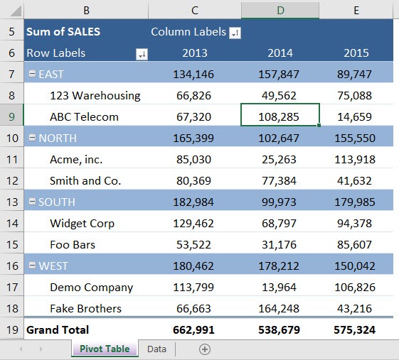
Inserting a Pivot Table is very easy to do in Microsoft Excel: Inserting a Pivot Table
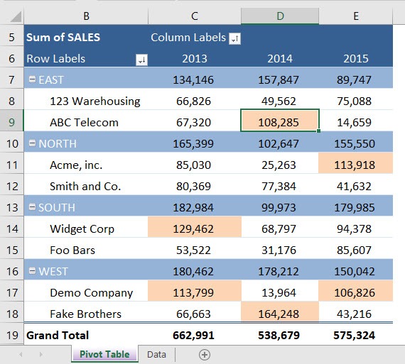
Adding some Conditional Formats to the Pivot Table allows a user to highlight key data in a split second.
See how easy it is to add some color to your analysis.
download workbookCond-Format-a-Pivot-Table.xlsx
STEP 1: We want to create a rule that will highlight values greater than 100,000
Select any cell inside the Pivot Table
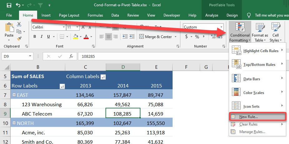
STEP 2: Go to Home > Conditional Formatting > New Rule
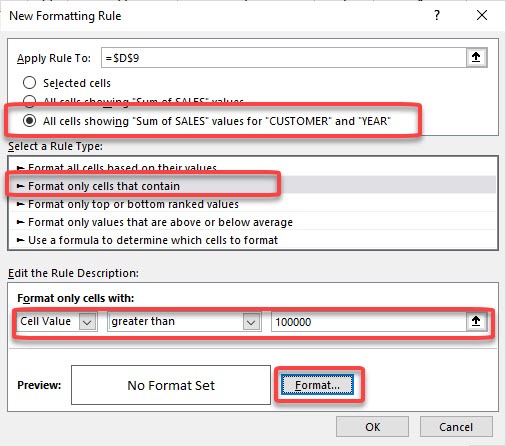
STEP 3: Select the following settings. We are selecting the third option so that the formatting rules only apply to the individual cell values
Click Format
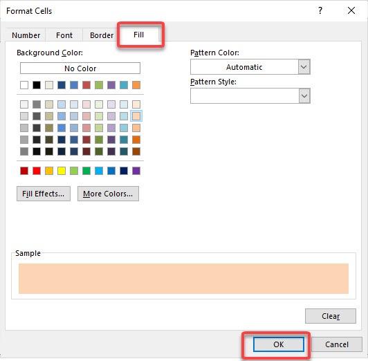
STEP 4: Select Fill and pick a color of your choice
Click OK twice
The formatting rule is now applied to your entire Pivot Table!
Helpful Resource:
John Michaloudis is a former accountant and finance analyst at General Electric, a Microsoft MVP since 2020, an Amazon #1 bestselling author of 4 Microsoft Excel books and teacher of Microsoft Excel & Office over at his flagship Academy Online Course.

