In this article, you will be covering the two methods for incorporating Power Query IF statement in Excel –
Download the Excel Workbook below to follow along and understand How to Write Power Query IF Statement in Excel –
download excel workbookPower-Query-IF-Statement.xlsx
Let’s dive into the practical applications of the Power Query IF statement.
Method 1 – Using Conditional Column
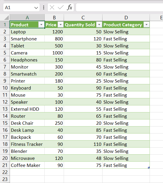
In Power Query, you can add a conditional column to apply a condition and determine the corresponding value. Let’s consider an example where we categorize products as “Fast Selling” or “Slow Selling” based on the quantity sold.
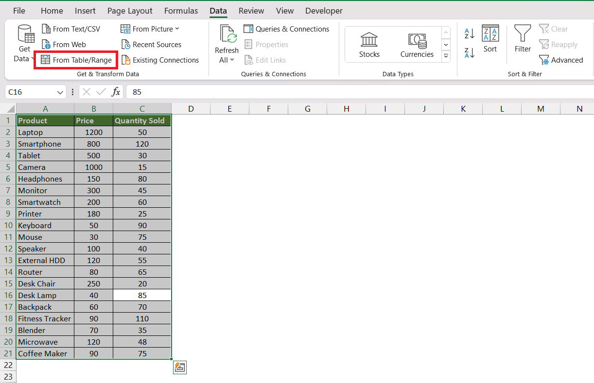
Suppose you have a list of products with the quantity sold listed in a data table. If the quantity sold is greater than 50, the product category will be fast selling else slow selling. Follow the steps below to add a conditional column in Power Query –
STEP 1: Highlight the data table and go to Data and select From Table/Range.
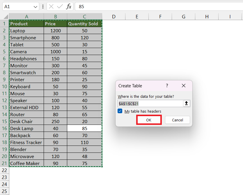
STEP 2: In the Create Table dialog box, select OK.
STEP 3: In the Power Query window, go to Add Column > Conditional Column.
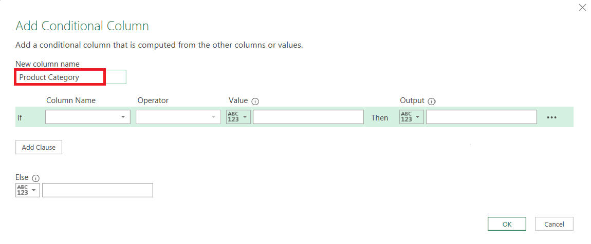
STEP 4: In the Add Conditional Column dialog box, name the new column “Product Category.”
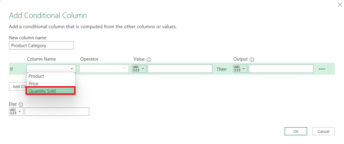
STEP 5: Set the column name to “Quantity Sold”
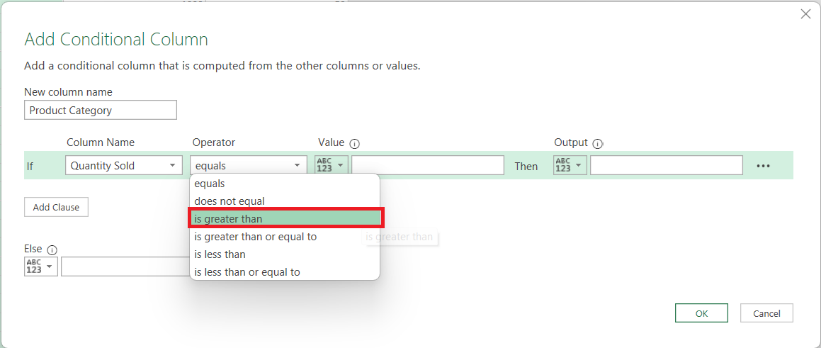
STEP 6: Choose the operator as “is greater than”.
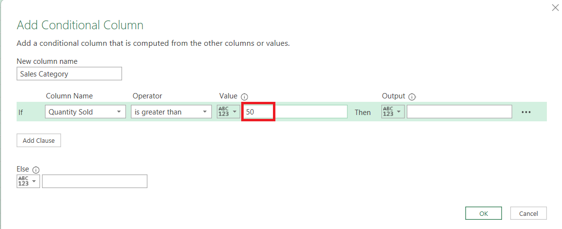
STEP 7: Enter the value as 50.
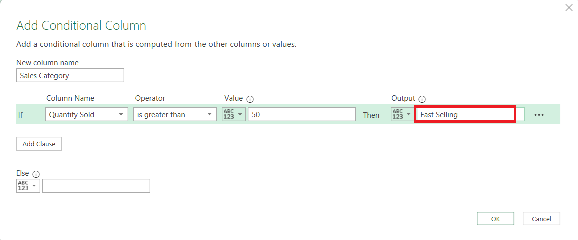
STEP 8: Specify the output as “Fast Selling”.
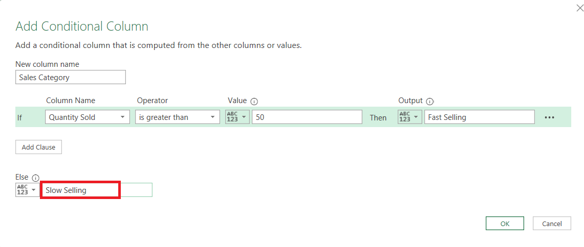
STEP 9: Enter “Slow Selling” as the Else value.
STEP 10: Finally, go to Home and select Close & Load.
This loads the data, now with the new conditional column, back into the Excel workbook.
Method 2 – Using Custom Column
Alternatively, you can write the IF statement in Power Query similarly to how you write an IF function in Excel. The syntax is as follows:
if condition then value1 else value2
where,
- condition – represents the logical test
- value1 – result if the condition is true
- value2 – result if the condition is false
Let us look at an example to understand better.
You can use Power Query IF statement to categorize these products based on the quantity sold using the syntax below –
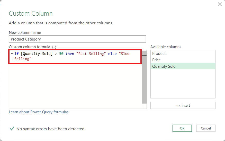
= if [Quantity Sold] > 50 then “Fast Selling” else “Slow Selling”
Follow the steps below to achieve this –
STEP 1: Highlight the data table and go to Data and select From Table/Range.
STEP 2: In the Create Table dialog box, select OK.
STEP 3: In the Power Query window, go to Add Column > Custom Column.
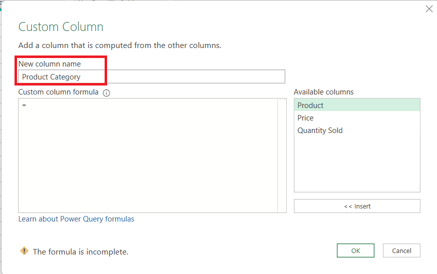
STEP 4: In the Custom Column dialog box, enter Product Category as the New column name.
STEP 5: Enter the following in the Custom column formula –
=if [Quantity Sold] > 50 then “Fast Selling” else “Slow Selling”
Click OK.
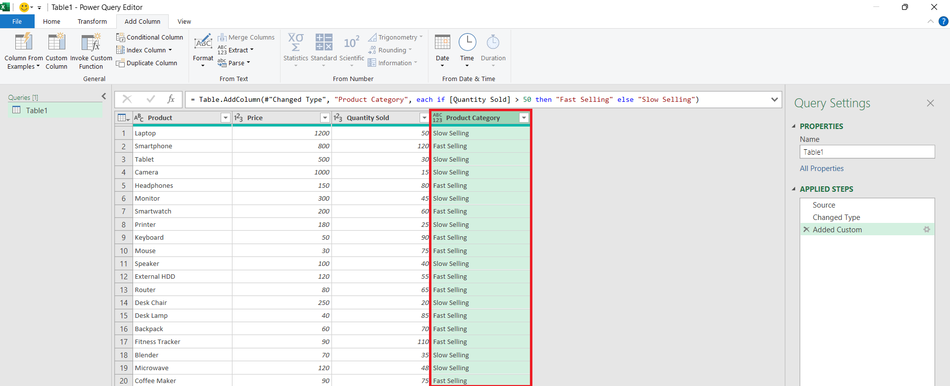
The new custom column will be added in the Power Query window.
STEP 10: Go to Home and select Close & Load.
This will load the data with the new custom column into the Excel workbook.
Please note the following –
- Power Query is case-sensitive, so you need to write “if”, “then”, and “else” in lowercase.
- There’s no need for a comma to separate value1 and value2.
- You can insert null if you want a result to be blank.
Conclusion
In a nutshell, Power Query in Excel is like a power tool for dealing with messy data. We learned two cool ways to use the IF statement – one by adding a special column based on conditions, and another by creating a custom column with a simple formula. Now, you can impress Excel with your data-handling skills!
Click here to learn more about Power Query in Excel.
John Michaloudis is a former accountant and finance analyst at General Electric, a Microsoft MVP since 2020, an Amazon #1 bestselling author of 4 Microsoft Excel books and teacher of Microsoft Excel & Office over at his flagship Academy Online Course.
