Predetermined Number Formatting in Excel Pivot Tables

What happened? Why did your formatting not take effect on the second sales column? I have the perfect workaround for adding predetermined number formatting in Pivot Table. Read on below!

Exercise Workbook:

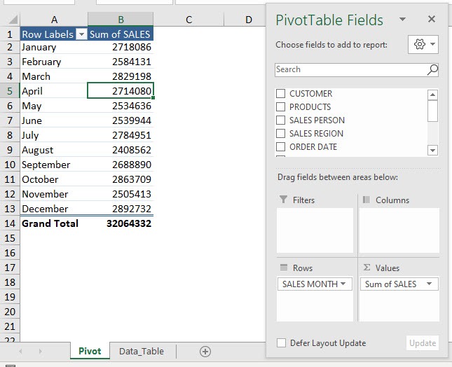
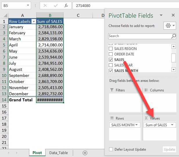
Here is our current Pivot Table setup:

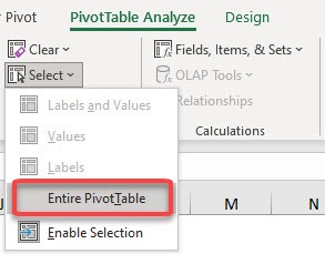
STEP 1: Let us select the entire Pivot Table. Go to PivotTable Analyze > Actions > Select > Entire PivotTable

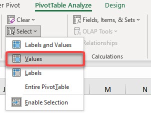
STEP 2: Now to select the sales numbers column, go to PivotTable Analyze > Actions > Select > Values

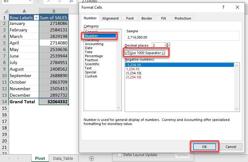
STEP 3: Let us apply our number formatting! Open the Format Cells dialog by pressing CTRL + 1

Select Number and tick the Use 1000 Separator (,)

Click OK

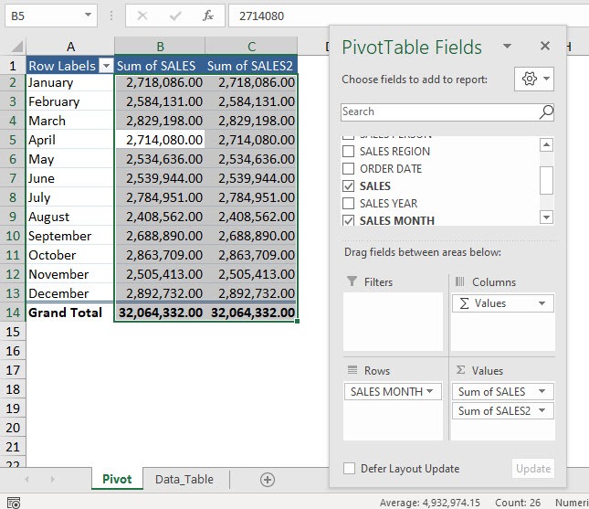
STEP 4: The number formatting is applied on our first Sales column. Now drag SALES to Values

The formatting is also applied to our second Sales column!

Bryan

Bryan is a best-selling book author of the 101 Excel Series paperback books.