Project Management is no easy feat! There are lots of moving parts, long hours, and constant reporting.
It requires you to keep everybody on the same page and focused on the goals and timelines.
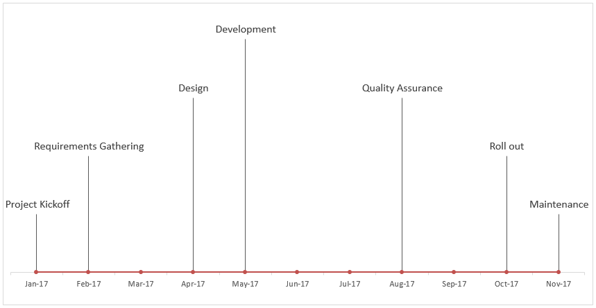
One of the key reporting tools needed is the project timeline or milestone chart. Luckily you can create a project milestone chart in Excel in just a few steps…well, 11 to be exact!
A milestone chart is used to keep track of your project with completion dates for various key checkpoints. It allows you to understand the scheduling of your project and all other information in a single chart!
Now, without any further delay let’s learn how to create a Milestone Chart in Excel!
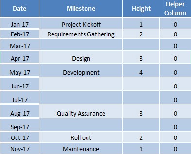
Below is the data source that we are going to use to create our timeline of milestones in Excel:
We have Dates and Milestones. The Height specifies how high we want the milestone to show up in the chart, whilst the Helper Column is used to create the timeline.
In this example, I show you how easy it is to insert a Milestone Chart Excel.
NB: This tutorial was made for Excel 2013 and Excel 2016 versions.
Follow the step-by-step tutorial on Milestone Chart in Excel and download this Excel workbook to practice along:
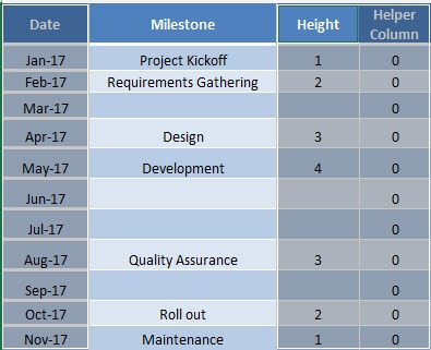
STEP 1: Highlight the following columns: Date, Height, and the Helper Column. You can select the 3 of them by holding the Ctrl button while highlighting them:
STEP 2: Go to Insert > Line Charts > Line with Markers
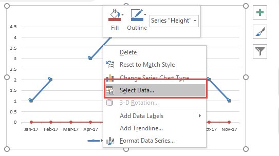
STEP 3: Right-click on your chart template and choose Select Data.
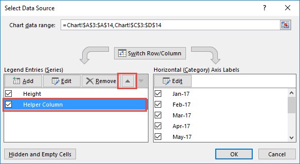
STEP 4: Select the Helper Column and press the Up arrow to move it up in order and press OK.
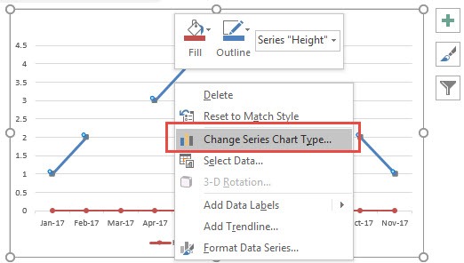
STEP 5: Select the Blue Lines (Height) & Right Click & select Change Series Chart Type.
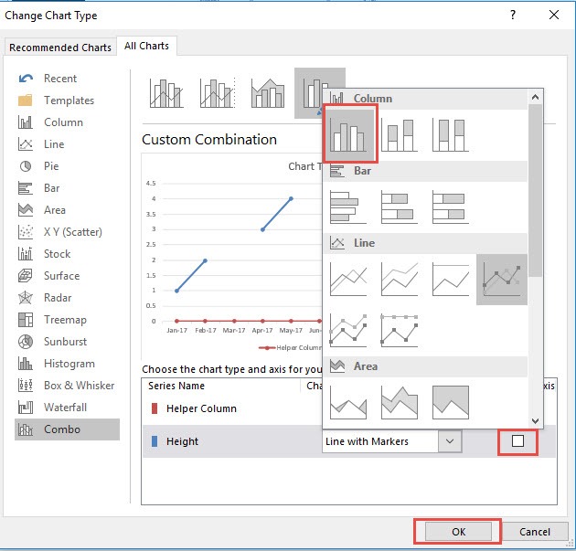
STEP 6: Under the All Charts tab, select the Combo chart.
From the Height drop-down, select the Clustered Column chart type and “check” the Secondary Axis box.
From the Helper Column drop-down, select the Line with Markers chart type and “uncheck” the Secondary Axis box.
Press OK to confirm.
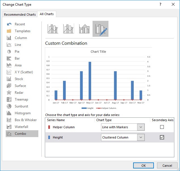
The reason we are doing this is so that our heights would now show up as columns in our timeline.
The selections should look like this:
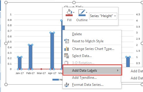
STEP 7: Select the blue column chart & right click & select Add Data Labels.
The magic is about to happen!
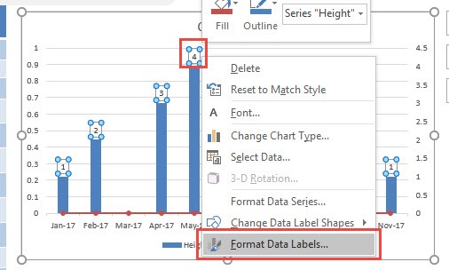
STEP 8: The height numbers will show up, however we do not need the height numbers to show up.
Select any one of the height numbers, right click and select Format Data Labels.
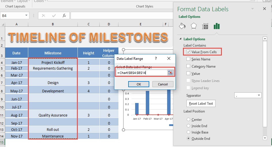
Under the Label Options (first icon from the right), make sure that only the Value From Cells is selected and the other boxes are deselected.
The Label Position should be Outside End.
Then highlight the Milestone values from the data source and press OK.
This will ensure that the Data Labels will be the Milestone text instead, which is what we want our timeline to show.
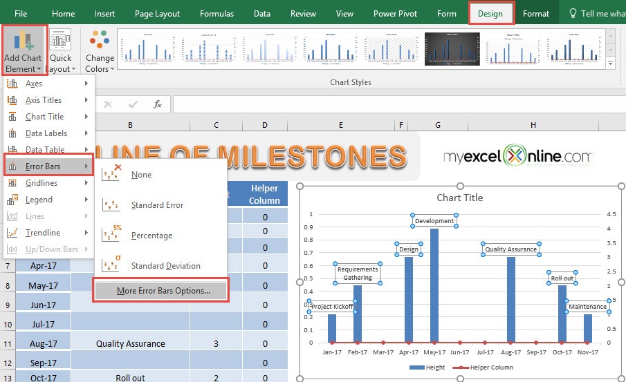
STEP 9: Now we will change the columns into thin lines. For this we will use the Error Bars.
Click anywhere on the chart template.
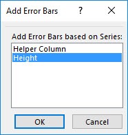
Go to Design > Add Chart Element > Error Bars > More Error Bar Options
Select Height. Click OK.
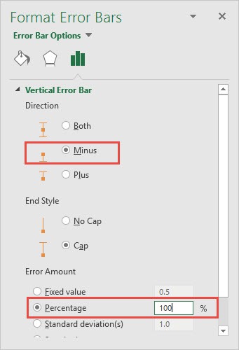
From the Format Error Bars pane on the right hand side of your workbook, make sure the Error Bar Options (first icon from the right) is selected and choose the:
Direction = Minus
End Style = Cap
Error Amount = Percentage at 100%.
This will ensure we have thin lines go all the way down the x-axis.
STEP 10: Now that we have the thin lines inside the column chart, let us remove the blue columns.
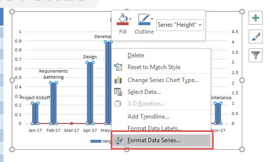
Right click on the blue column chart and select Format Data Series.
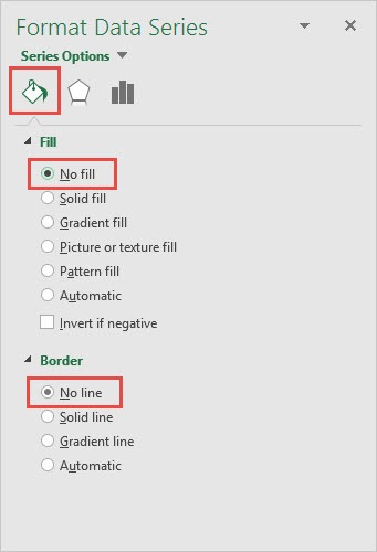
From the Format Data Series pane, select the Fill bucket (first icon from the left) and make sure that the following are selected:
Fill = No fill
Border = No line
STEP 11: And now for the finishing touches!
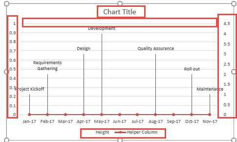
Let us delete the unnecessary labels in our chart to make it look nicer. Just click on each element and press the Delete key from your keyboard.
And there you have it! Your own Timeline of Milestone Chart is ready!
These charts are extremely useful in displaying key milestones or major achievements of a project in a graphical manner. They are easy to understand and self-explanatory!
Feel free to change the data source so you can see how your cool new Timeline chart changes. Happy project managing using Excel!
HELPFUL RESOURCE:
Make sure to download our FREE PDF on the 333 Excel keyboard Shortcuts here:
Bryan
Bryan is a best-selling book author of the 101 Excel Series paperback books.
