Excel Pivot Tables have a lot of useful calculations under the SHOW VALUES AS option and one that can help you a lot is the Excel Pivot Table RANK LARGEST TO SMALLEST calculation.
This option will immediately calculate the rankings (1 being the LARGEST value) for your values, allowing you to pinpoint the risks or opportunities quickly!
It allows you to analyze data by ranking them and check what’s on top and what is at the bottom!
You can easily do ranking in Pivot Table using either of the two methods mentioned below:
Let’s look at these methods in-depth!
In the example below I show you how to get the Excel Pivot Table Rank Largest to Smallest:
Follow the step-by-step tutorial on Excel Pivot Table Rank Largest to Smallest and download this Excel workbook to practice along:
Using Sorting Option
STEP 1: Insert a new Pivot table by clicking on your data and going to Insert > Pivot Table > New Worksheet or Existing Worksheet
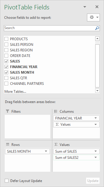
STEP 2: In the ROWS section put in the Sales Month field, in the COLUMNS put in the Financial Year field, and in the VALUES area you need to put in the Sales field twice, I explain why below:
STEP 3: Click the second Sales field’s (Sum of SALES2) drop down and choose Value Field Settings
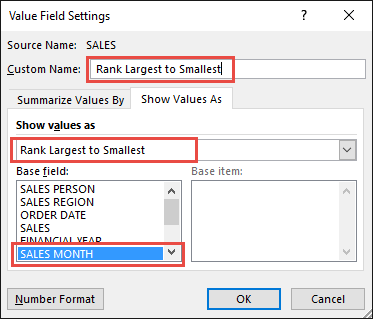
STEP 4: Select the Show Values As tab and from the drop down choose Rank Largest to Smallest.
Select Sales Month as the Base Field. This means that we will rank the Sales Values by the Sales Month (where Rank 1 is the Largest).
Also change the Custom Name into Rank Largest to Smallest to make it more presentable. Click OK.
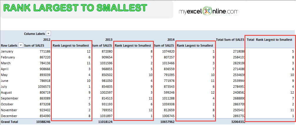
You now have your Pivot Table, showing the Rank Largest to Smallest for the sales data of years 2012, 2013, and 2014.
You can see that each red box is the ranking for each year (for Years 2012, 2013, 2014, and the Total Rankings).
This is how you can easily Rank Pivot Table in few easy steps!
Using Calculated Field
STEP 1: Select any cell in the data and then Go to Insert > Pivot Table.
STEP 2: In the dialog box, select New Worksheet and then click OK.
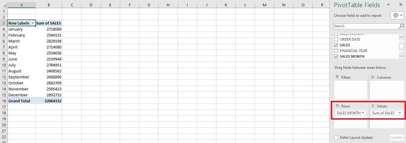
STEP 3: Drag and drop Sales Month in the Row field and Sales in the Values field.
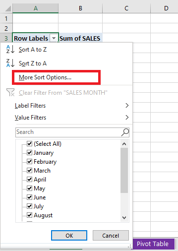
STEP 4: Click on the filter button and Select More Sorting Option.
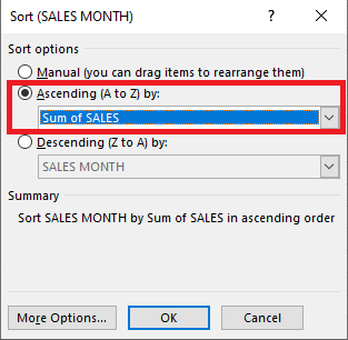
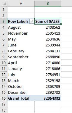
STEP 5: In the Sort dialog box, Select Sum of Sales in the Ascending by dropdown. Click OK.
This will sort the data in ascending order!
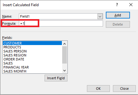
STEP 6: Click on any cell in the Pivot Table and Go to PivotTable Analyze > Calculated Field.
STEP 7: In the Insert Calculated Field dialog box, Type =1 n the formula field. Click OK.
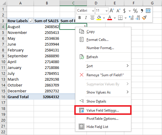
STEP 8: Right-Click on the calculated field and select Value Field Setting.
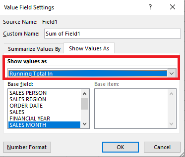
STEP 9: In the Value Field Setting dialog box, Select Running Total in as Show Value as! Click OK.
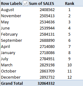
This will sort the values from largest to smallest and insert a rank field in the Pivot Table!
Conclusion
In this tutorial, you have learned how to rank in pivot table by either using the Sorting option or by inserting a calculated field.
Make sure to download our FREE PDF on the 333 Excel keyboard Shortcuts here:
Bryan
Bryan is a best-selling book author of the 101 Excel Series paperback books.


