Rank Smallest to Largest With Excel Pivot Tables

Excel Pivot Tables have a lot of useful calculations under the SHOW VALUES AS option and one that can help you a lot is the RANK SMALLEST TO LARGEST calculation.

This option will immediately calculate the rankings (1 being the smallest value) for your values, allowing you to pinpoint the risks or opportunities quickly!

In the example below I show you how to get the Rank Smallest to Largest:

download excel workbook Rank-Smallest-to-Largest.xlsx

STEP 1: Insert a new Pivot table by clicking on your data and going to Insert > Pivot Table > New Worksheet or Existing Worksheet

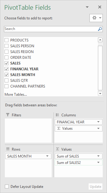
STEP 2: In the ROWS section put in the Sales Month field, in the COLUMNS put in the Financial Year field and in the VALUES area you need to put in the Sales field twice, I explain why below:

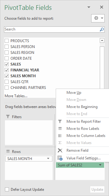
STEP 3: Click the second Sales field’s (Sum of SALES2) drop down and choose Value Field Settings

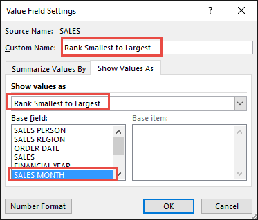
STEP 4: Select the Show Values As tab and from the drop down choose Rank Smallest to Largest.  

Select Sales Month as the Base Field.

This means that we will rank the Sales Values by the Sales Month (where Rank 1 is the Smallest).

Also change the Custom Name into Rank Smallest to Largest to make it more presentable. Click OK.

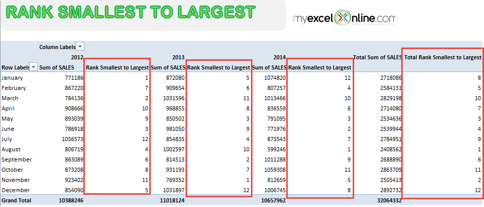
You now have your Pivot Table, showing the Smallest to Largest Rankings for each Month.

You can see that each red box is the ranking for each individual year (for Years 2012, 2013, 2014 and the Total Rankings).

Bryan

See also  Learn How to Use ChatGPT in Under 5 Minutes!

Bryan is a best-selling book author of the 101 Excel Series paperback books.