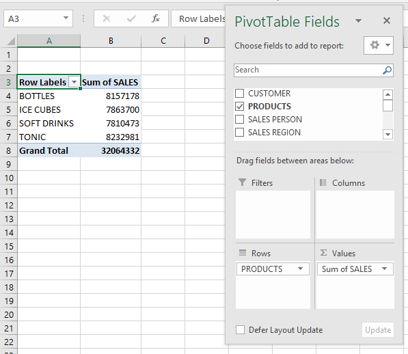
Did you know that Excel can automatically generate Pivot Tables for you? You heard that right, there are Recommended Pivot Tables in Excel that you can actually use!
This is a new feature introduced in Excel 2013.
It is very simple to do so and we will show you how!
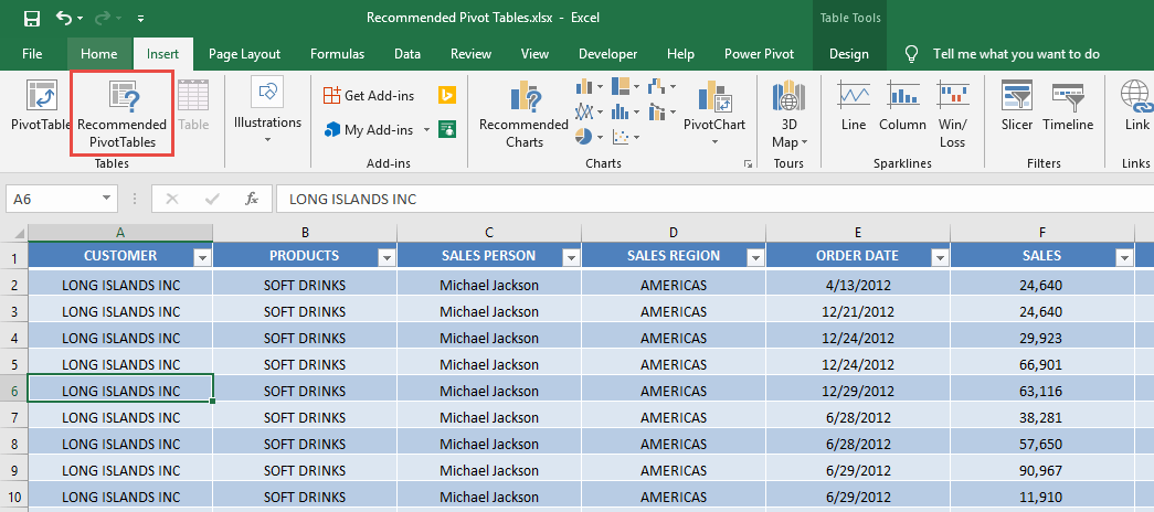
STEP 1: Make sure you have selected your data. Go to Insert > Tables > Recommended Pivot Tables
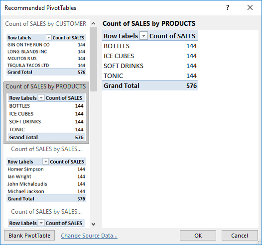
STEP 2: You will see the generated Pivot Table recommendations.
Let us select the Count of SALES by PRODUCTS. Click OK.
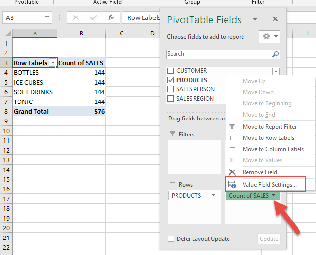
STEP 3: The generated Pivot Table is now in a new sheet. Let us make some changes to it.
Click on COUNT of SALES and select Value Field Settings.
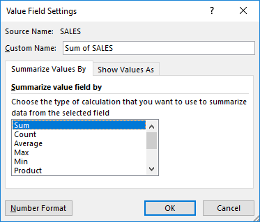
We want it to display the Total sum of Sales per Product instead. Select Sum and click OK.
With just that, your Pivot Table is now ready!
How to Use Recommended Pivot Tables in Excel
Bryan
Bryan is a best-selling book author of the 101 Excel Series paperback books.

